Structure and Interpretation

of Tensor Programs

First Edition

A Whirlwind Tour to Deep Learning and Deep Learning Systems
Runnanochatby buildingteenygradfrom scratch: the bridge from microgradto tinygrad
with the Lean, Python, Rust, and CUDA Rust programming languages!

Made with 🖤🪻 by Jeffrey Zhang, University of Waterloo (BMath)
Made possible by Lambda Labs Research Grant

Citation:

@book{zhang2026sitp,
  author = "Jeffrey David Zhang",
  title = "Structure and Interpretation of Tensor Programs",
  year = 2026,
  url = "https://sitp.ai"
}

Dedication

In loving memory of my father, my teacher, and my best friend Dr. Thomas Zhang ND., R.TCMP, R.Ac.
The love I put into this book is but a fraction of the love he gave me.
May you rest in pure land. We’ll meet again dad.

We’ll Meet Again by Vera Lynn 1939. Cover by Johnny Cash 2002.

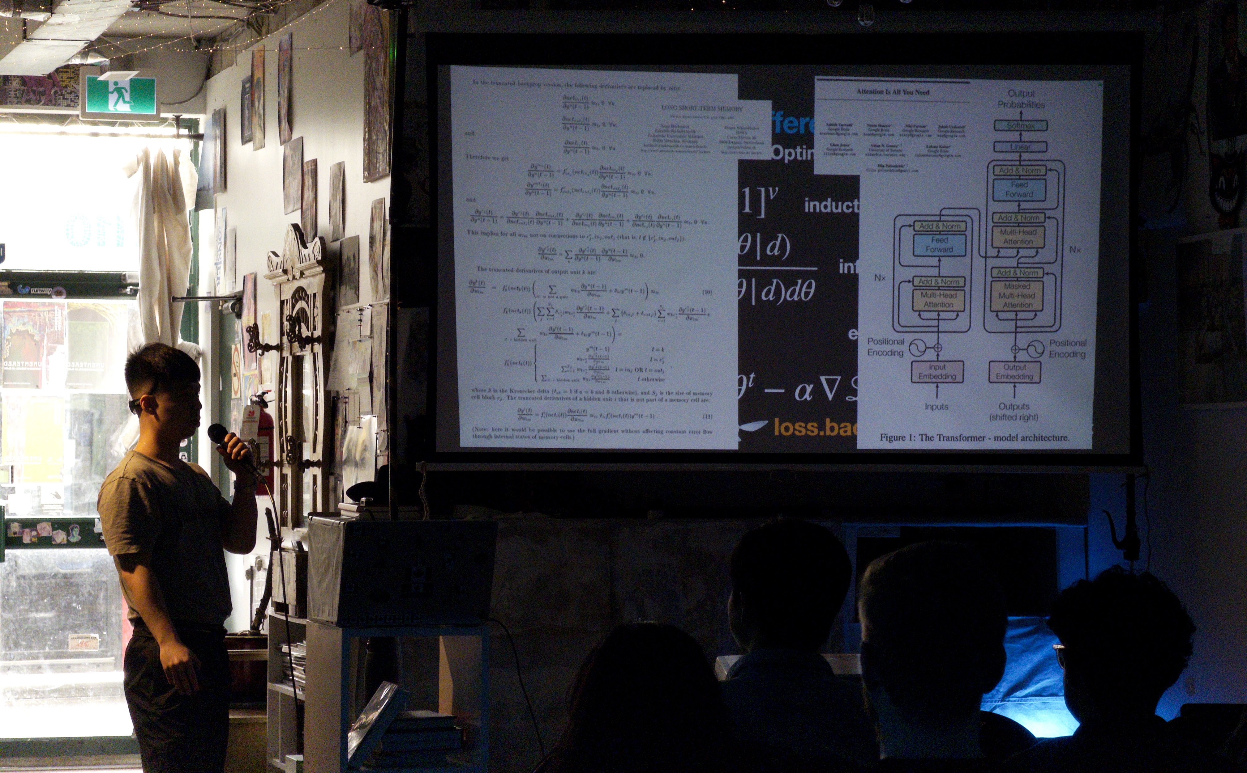Presenting an early outline of SITP at Toronto School of Foundation Modeling Season 1 (November 2025)

Preface

The Structure and Interpretation of The AI Curriculum

This book is aspirationally titled The Structure and Interpretation of Tensor Programs, (henceforth SITP) as it’s goal is to serve a similar role for software 2.0 as The Structure and Interpretation of Computer Programs (henceforth SICP) did for software 1.0. Written by Harold Abelson and Gerald Sussman with Julie Sussman, SICP took learners on a whimsical whirlwind tour throughout the essence of computation starting with the elements of programs with functional programming, higher order functions, data abstraction, streams, and ending with programming their own programming languages with interpreters, compilers, and register machines.

My alma matter was amongst those which took the SICP approachActually it’s Scheming dual, HtDP., and as intended, for someone coming into first year college with high school computer science, it blew my mind. After graduating college in 2022, I followed my curiosity for diving deeper into the souls of our machine by going on to developing industrial languages and runtimes.“There is only one project, architecture, operating system and languages, compiler, it’s only one project. It’s all together.” – Boris Babayan. Particularly, I hacked on languages with domain specific cloud compilers and runtimes with cloud provisioners, and cloud garbage collectors. At the end of 2022 though, when ChatGPT was released by OpenAI my mind was blown twice more. As someone programming since high school, I could not believe this at all. After two more years of hacking on cloud languages and runtimes, I started my transition from domain specific cloud compilers from GPS to Terraform to to domain specific tensor compilers from PyTorch to Triton.

The transition started with a tweet showcasing the beginnings of a tensor library evaluating the forward pass of a feed forward network from Andrej Karpathy’s Neural Networks: Zero to Hero course. While it was illuminating to start implementing each individual torch call that the nets from makemore were making, my knowledge felt quite fragmented as I personally forgot a lot of the foundational mathematics and I wasn’t sure how to bridge myself to industrial deep learning systems like tinygrad, torch, jax, vllm, and sglang.

Shortly after, I decided to take the plunge and started drinking from the firehose of deep learning canon: Hastie et al.,, Murphy, Goodfellow et al.,, you name it. The one thought I could not get out of my head was where is the SICP for software 2.0? While I found two excellent resources on building your own torch-like autograd by Tianqi Chen at Carnegie Mellon and Sasha Rush at Cornell, I personally would have enjoyed a unified resource that took me from math, to deep learning, to deep learning systems in a single unbroken sequence of thought, and perhaps others would feel similarly. That is the genesis story for this book, whose central research question is the following: What does the SICP for Deep Learning look like?

Jeffrey Zhang
Waterloo, Ontario
August 2026

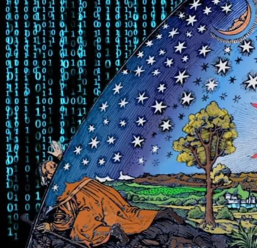
Frontispiece of Dialogue Concerning the Two Chief World Systems (Galileo Galilei 1632)

WeA modified excerpt from The Structure and Interpretation of Computer Programs §1: Building Abstractions with Procedures are about to study the idea of a computational process. Computational processes are abstract beings that inhabit computers. As they evolve, processes manipulate other abstract things called data. The evolution of a process is directed by a pattern of rules called a program parameters called a model. People create programs train models to direct processes. In effect, we conjure the spirits of the computer with our spells.

A computational process is indeed much like a sorcerer’s idea of a spirit. It cannot be seen or touched. It is not composed of matter at all. However, it is very real. It can perform intellectual work. It can answer questions. It can affect the world by disbursing money at a bank or by controlling a robot arm in a factory. The programs models we use to conjure processes are like a sorcerer’s spells. They are carefully composed recovered from symbolic numerical expressions in arcane and esoteric parallel programming languages that prescribe the tasks losses we want our processes to perform minimize.

I. Elements of Networks

Not different from learning another mathematical or programming language, they must transition from their finitely discrete structures and deterministic procedures tooling they have grown acustomed to and make the transition to the infintely continuous structures and stochastic procedures. Back then, ancient greek mathematicians were only comfortable with the finiteness of natural numbers like $1$, $2$, and $3$, and had to grapple with the infinite nature of the real numbers such as $\sqrt{2}$, $\pi$, and $e$. Similarly, the programmers of today are being asked to transition from programming algorithms of sets, maps, lists, trees, and graphs to the distributions of scalars, vectors, matrices, tensors, and neural networks.

More coloquially, programmers interested in the deep learning approach to artificial intelligence must make the transition from software 1.0software 1.0 to software 2.0software 2.0 See (Karpathy 2017), a distinction used to differentiate the classical act of programming software line by line, and the newer approach of programming software by specifying a dataset, a neural net architecture with a goal, and searching the space of programs with compute. How to exactly program with this new approach will take the remainder of the book to explain.

While software 2.0 has increased the intelligence and autonomy of our devices throughout the past decade — to name a few, language understanding with Google’s Translate and Apple’s Siri, vision understanding with Tesla Autopilot — at the end of 2022 ChatGPT was released to the world marking the beginning of software 3.0software 3.0 See (Karpathy 2025), enabling the activity of programming with none other than the English language. What may be surprising to realize is that artificial intelligence like ChatGPT is “just” another computer program. However, rather than being implemented in a language like C, Java, or Javascript, it’s implemented in one that goes by the name of PyTorch, a software 2.0 programming language centered around torch.Tensor, a multidimensional array humbly embedded within a Python package.

In this whimsical whirlwind tour dubbed The Structure and Interpretation of Tensor Programs (SITP), we will embark on a quest to build from scratch our own deep neural network like ChatGPT by implementing nanochat and our own deep learning framework like PyTorch by implementing teenygrad. Whether you’re an eager high school student, an up coming college student, or a battle-tested industry programmer, SITP has been meticulously designed so that the only prerequisite required is a basic familiarity with the elements of programming, and high school calculus. Any additional experience is helpful, not mandatory.

So with that all said, go on young hacker. Venture forth!

Table of Contents

Overture: A Lean Snake and Parallel Crab

In which we introduce and motivate the programming languages used throughout the book, including Lean, Python, Rust, and CUDA Rust.

The primary story this book tells is the one of how intertwined the activities of mathematics and programming are with respect to the discipline of deep learning. That is, the performance of the systems in which neural networks are trained on affect bottom line quality as much as their architectures. As a first approximation, you can conceptualize deep learning frameworks like torch and jax as Python packages that provide accelerated, mathematical primitives of statistical distributions, high dimensional arrays, and optimizers from probability theory, linear algebra, and calculus.

In SITP however, you will be using a framework called teenygrad, which you can roughly think of a minimal, hackable subset that avoids the complexity and cost that the more industrial frameworks offerAfter our journey together, you can take a look at the Afterword which explains the primary differences between such frameworks, thus bridging you from teenygrad to torch and jax.. In addition, not only will you be using teenygrad but also implementing your very own. By the end of the book, you will have a working implementation of teenygrad capable of running distributed training and inference for nanochat, which you are encouraged to modify, extend, and hack on thereafter. This is effectively the primary purpose of this book: for you to learn deep learning and deep learning systems in one unified treatment, which brings us to our next order of business: presenting the show’s cast with a playbill, or in other words, the map of the territory.

In order to provide accelerated mathematical primitives, deep learning frameworks (including teenygrad) are implemented with a variety of programming languages. For teenygrad specifically, we will be using four, namely that of the Lean, Python, Rust, and CUDA Rust programming languages. Such languages are referred to as host languages because they are used to implement the teenygrad deep learning language. We briefly motivate each language, explain the order in which they will be presented, suggest possible reading “passes” to iteratively and incrementally deepen your use of each language, and provide alternatives.

First, Python is of course used because that is the primary programming language in which artificial intelligence community conducts its research in, and for good reason. It’s an extremely productive one, especially for researchers who might be not as well versed in the dark arts of casting spells upon the computer. The first contact of any mathematical concept will be an intuitive and informal one, using teenygrad in Python in order to carry out a computation. Then, the second contact is in between chapters with Intermezzos, which formalize those very same concepts using dependent types provided by the interactive proof assistant Lean. These intermezzos can optionally be skipped upon a first reading. However, each successive chapter will assume and make use of the formalized concepts within each Intermezzo therein.

The third and fourth contact of a given mathematical concept are in tandem, which involves implementing teenygrad in a mix of the Python, Rust, and CUDA Rust programming languages. Systems programming languages like Rust and CUDA Rust are used in order to provide native acceleration of multi and massively parallel processors like CPUs and GPUs. For each mathematical concept, a slower version will be implemented with a mix of Python and Rust, and a faster version will be implemented with CUDA Rust.

If you find yourself more mathematically oriented and disinterested in the high performance computing and performance engineering of such mathematical primitives, you can skip any sections with CUDA Rust, and implement the sections using Rust with Python. If you find yourself inclined in such peformance engineering but are not interested in learning the Rust and CUDA Rust programming languages, you can follow along with C/C++ and CUDA C/C++, although the primary difference not much, given that Rust’s ownership is simply formalizing many of the language features of C++11 with linear types. If you find yourself interested in the performance engineering but disinterested in both Rust and C++, you can use CUDA Python.

We surface all this complexity now because we trust you to make the right decision for yourself. If you want to follow along with a pure Haskell implementation, go for it. Take charge of your own education, as ultimately you are the captain of your own ship. This is no different to professors and authors that offer courses and textbooks on compiler construction provide the freedom for learners to choose the host language you will use for your compiler — they are assuming that what is new to you is not the host language, but the principles of compiler construction itself. Similarly, this book is emphatically not about teaching any of the aforementioned four languages, but rather the principles of deep learning and deep learning systems. That is, these various programming languages are the means of SITP rather than the end.

With that being said, we briefly provide a unified introduction the three programming languages of Lean, Python, and Rust together so you can compare and contrast with the foundation you already have as a programmer in §A. From Problems to Proof, which constructs various number systems along with some elementary proofs.

With that said, down the rabbit hole we go.

1. Self-Supervised Sequence Learning with Single-Layer Networks

$\hookleftarrow$ Table of Contents

In which we transition to the stochastic and infinitely continuous software 2.0 by implementing ngram and linear language models with teenygrad using the languages of probability theory, linear algebra, and calculus.

1.1 From Certain to Uncertain Knowledge

$\hookleftarrow$ Table of Contents

Although ChatGPT, Claude and friends are relatively new to our universe, the idea of generating sentences with next token prediction is surprisingly not new and dates back to the work of Russian mathematician Andrey Andreyevich Markov in 1913, and shortly after Claude Shannon in 1948Will the real Claude please stand up?. So why is humanity’s so-called tech tree late to such technology? Predominantly for two reasons.

Philosophically, because of the eternal tension between the discretediscrete and continuouscontinuous methods in describing our reality. Programmers were reluctant to use stochastic and infinitely continuous techniques, favoring those that were logical and finitely discrete. However, … like a physicist position of every particle in a vacuum, even with a set of initial equations for position and momentum with equations for change, bitter lessondescribing reality with too many parts to count. This created the need for statistical mechanics, describing particles with probability distributionsprobability distributions.

Practically, it’s predominantly because of the fossil-fuel like subsidy of datadata provided by the aforementioned intergalactic computer network we call the web, the computecompute provided by massively parallel processors originally designed for video games we call graphic processing units (henceforth GPUs), which can be used efficiently by a neural network architecturearchitecture called attention. This is why ChatGPT Claude are called large language modellarge language models.

Large Language Models explained briefly (Grant Sanderson, 3Blue1Brown 2024)

Large language models are trained using methods from the discipline of deep learningdeep learning, which in turn, are based in the statistical machine learningmachine learning approach to artificial intelligence. This means, in order to produce such a probability distribution over possible next words, ChatGPT, Claude and others use a lot of mathematical machinery from the areas of probability theory (clearly), linear algebra, and calculus. We will introduce such mathematical primitives by keeping our language models simple at first in Part I. Elements of Networks — namely what is called the ngram model and linear models in which the aforementioned Markov and Shannon were working on around a century ago — before diving into the design of neural network architectures (including transformers with the attention operator) in Part II. Deep Neural Networks.

Note

If you’d like a more historical and philosophical approach in how the logical and finitely discrete techniques of software 1.0 failed to build such conversational machines, you are encouraged to visit §B. From Symbolic Software 1.0 to Stochastic Software 2.0, which covers early systems from classical computational linguistics and natural language processing. Namely, ELIZA, LUNAR, and CYC.

Up ahead we will be intuitively introducing many notions from probability and linear algebra in the context of large language modelling with numpy. At any time you find yourself interested in the formal definitions of such concepts — whether before the intuition pump, in between, or after —, you can encouraged to visit §Intermezzo One: The Language of Probability and Linear Algebra.

Consider the partial sentence “Hello world, nice to” and feed it into GPT-2 with the words “meet you” missing. When you click the button “predict”, GPT-2 produces a list of real numbers approximately represented by floating points that are between 0 and 1 and sum (or normalize) to 1, which is called a distributiondistribution, because it is distributing truth across a weighted set of values, on in other words, it’s uncertaintyuncertainty. Each number represents the probabilityprobability, chancechance, likelihoodlikelihood, or beliefbelief that GPT-2 assigns to an outcomeoutcome, which in this case is the next word.

But rather then produce a distribution with two outcomes like a coin, six outcomes like a die, or fifty two outcomes like cards, it produces one for $|V|$ outcomes, where $V$ is the set of words in some vocabulary. The size of GPT-2’s vocabulary is 50257, and the list of probabilities you see in Demo 1.1 are the top 10 most likely. As a first approximation, it’s not incorrect to conceptualize large language models as an urn containing a ball labeled with each word in the vocabulary. However, it’s important to note in the case of language that some balls are weighted heavier than others.

To be more precise, because we are passing an input sentence, such a distribution is a conditional distributionconditional distribution. That is, GPT-2 is producing the distribution of the next word conditioned on the sequence of words passed in as input, and is denoted by

$p(w\underset{\text{given}}{\underbrace{|}}\text{input sentence})$

and with Demo 1.1, you are asking GPT-2 to produce $p(w|\text{Hello world, nice to})$. More accurately, each number in that list of probabilities is the chance that GPT-2 assigns a random variablerandom variable taking on outcome. A random variable is like a deterministic variable in that it can take on values, but it can possibly take on many at a single time, and are thus correspond to a distributed array of values which we call a distribution. We can print the conditional distribution that GPT-2 produces given the history $\text{Hello world, nice to}$

import numpy as np

# The same GPT-2 output distribution p(w | "Hello world, nice to") from above, top 10 of 50257 words
tokens = ["see", "meet", "hear", "have", "be", "know", "you", "talk", "say", "get"]
probs = np.array([0.3169, 0.1268, 0.1246, 0.1046, 0.0471, 0.0352, 0.0320, 0.0128, 0.0114, 0.0067])

print("Asking GPT-2 what is p(w|Hello world, nice to):")
for i in np.argsort(-probs):
    print(f"{tokens[i]} : {probs[i]:.4f}")
print(f"Total sum of p(w|Hello world, nice to): {probs.sum():.4f}")

Every random variable is endowed with a distribution, and you can conceptualize the probs distribution as the random variable, because it distributes the truth or state of the next word across a vocabulary of 50257 words. Each index i of the probs array corresponds to a value in the token outcomes tokens[i], with each probs[i] corresponding to the chance, possibility, of the random variable taking on the value tokens[i]. That is, probability is conducted with weighted array of values indexed by i. The type of a distribution $p$ is some function $p:\mathbb{N}\to [0,1]$ that sends indices to their probabilities, such that for all $n\in \mathbb{N},p(n)\ge 0$ and $\sum _{n\in \mathbb{N}}=1$. (todo: refine type of domain?)

Important

Probability can be seen as array programming! Every valid distribution which is some function $p:\mathbb{N}\to [0,1]$ whose values are between 0 and 1 and normalizes to 1 has a corresponding np.ndarray with .shape of (todo).

To make random variables more explicit, some people will denote distributions with them included, which in our case of a conditional distribution over next words, is $p(W=w|H=\mathbf{h})$ or $p_{W|H}(w|\mathbf{h})$. However, this brings us to our next point which is that with conditional distributions, the random variable being conditioned on is actually no longer random, because it is assumed that it has already taken on a value, in this case $\mathbf{h}\in {\mathbb{R}}^4$ where ${\mathbf{h}}_0=\text{Hello}$, ${\mathbf{h}}_1=\text{world}$, ${\mathbf{h}}_2=\text{nice},{\mathbf{h}}_3=\text{to}$. So, with $p(w|\mathbf{h})$ more generally, there is no randomness associated with the history $\mathbf{h}$.

We can validate that such a distribution $p(w|\mathbf{h})$ is valid distribution by verifying that each probability is between 0 and 1 and the distribution normalizes to 1. However, since we are only including the top 10 most likely words out of 50256, the total sum of probs is 0.8181, with the other 1-0.8181=0.1819 spread amongst the other 50256-10=50246 unseen words.

You may have also noticed that the output distribution is not a vanilla Python list, but rather one initialized with np.array, which constructs the multidimensional arraymultidimensional array np.ndarray. While we will gradually become more intimately familiar with mutldimensional arrays such as np.ndarray throughout the course of this adventure, as a first approximation multidimensional array’s are simply what they say on the tin can. 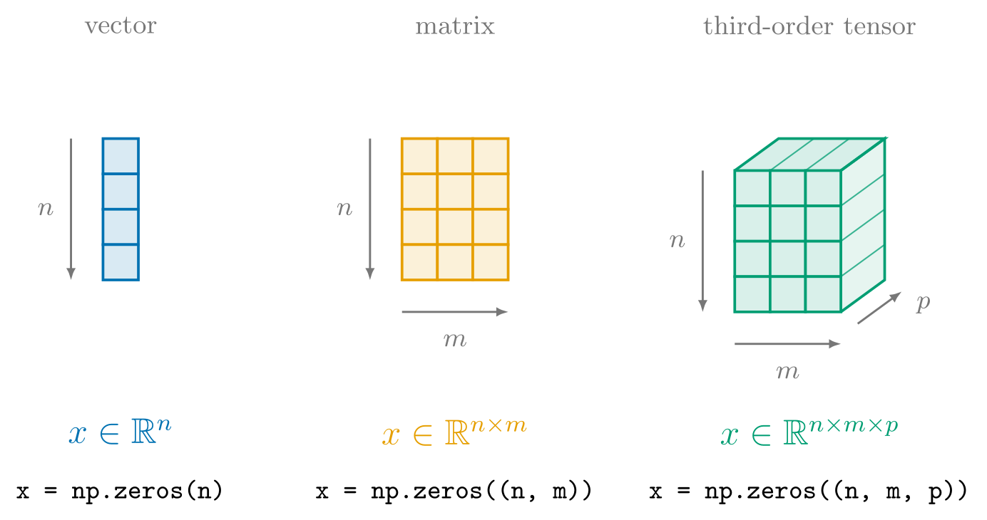That is, they are arrays with multiple rankdimensions, enabling the representation of scalarscalars, vectorvectors, matrixmatrices, and arbitrary tensortensors of arbitrary rank. In the case of probs, it’s a vector with support in ${\mathbb{R}}^{|V|}$, which we can verify with the two key properties of an ndarray, namely ndarray.shape and ndarray.dtype:

import numpy as np

# The same GPT-2 output distribution p(w | "Hello world, nice to") from above, top 10 of 50257 words
tokens = ["see", " meet", " hear", " have", " be", " know", " you", " talk", " say", " get"]
probs = np.array([0.3169, 0.1268, 0.1246, 0.1046, 0.0471, 0.0352, 0.0320, 0.0128, 0.0114, 0.0067])

print("gpt-2's output distribution is stored with an np.ndarray rather than a vanilla python list")
print(f"probs.shape {type(probs.shape)}: {probs.shape}")
print(f"probs.dtype {type(probs.dtype)}: {probs.dtype}")

my_tuple = (3, 4, 5)
my_tuple[0] = 2

TypeError: 'tuple' object does not support item assignment

x_reshape.shape, x_reshape.ndim, x_reshape.T

((2, 3),
 2,
 array([[5, 4],
        [2, 5],
        [3, 6]]))

np.sqrt(x)

array([2.24, 1.41, 1.73, 2.  , 2.24, 2.45])

Where .shapeprobs.shape and .dtypeprobs.dtype evaluating to (10,) and dtype64 respectively means it’s a vector with support in ${\mathbb{R}}^{10}$ whose real values are being approximately represented with double precision floating point numbers. Another important attribute is .ndimndarray.ndim, which is len(probs.shape) and reports the rank of an array. Since probs.ndim evaluates to 1, it has a rank of 1, or equivalently, is a vector.row major (todo)row major (todo) col major (todo)col major (todo) (todo, resulting tensor from .reshape() aliases the same underlying storage with different shape and strides. )

Warning

A 10-dimensional vector is some ${\mathbf{x}}^{(1)}\in {\mathbb{R}}^{10}$. A 100-dimensional vector is some ${\mathbf{x}}^{(2)}\in {\mathbb{R}}^{100}$. Both vectors ${\mathbf{x}}^{(1)}$, and ${\mathbf{x}}^{(2)}$, have a rank of 1, hence why they are both considered vectors. Unfortunately with numpy a rank is stored under the ndarray.ndim attribute.

So, an array whose ndarray.ndim evaluates to 2 is not some vector ${\mathbf{x}}^{(3)}\in {\mathbb{R}}^2$ but rather, an array that is some matrix ${\mathbf{x}}^{(4)}\in {\mathbb{R}}^{n\times m}$, where $n$ and $m$ are unknown since ndarray.shape was not supplied. Conversely, a multidimensional array is not simply a flat array with arbitrary length $n$ to corresponding to any vector in ${\mathbb{R}}^n$, but rather an array with arbitrary rank $n$ corresponding to any tensor ${\mathbf{x}}^{(4)}\in {\mathbb{R}}^{d_1\times d_2\times \cdots \times d_n}$. That is, multidimensional arrays are more accurately described as multirank arrays!

Returning to the focal point of probability and GPT-2’s conditional distribution $p(w|\mathbf{h})$, we now know that it corresponds with an ndarray whose .shape is (50256,), or in other words some vector $\mathbf{x}\in {\mathbb{R}}^{50256}$. More generally, an ndarray with .shape of (V), corresponds to a vector with a support $\mathbf{x}\in {\mathbb{R}}^{|V|}$, where $V$ is the vocabulary. (todo: context-length is dimensionality of $\mathbf{h}$). For convenience sake, we analyzed the top 10 probabilities with an ndarray whose .shape was (10,), which corresponded to a vector $\mathbf{x}\in {\mathbb{R}}^{10}$.

outcomes -> events

• todo eventevent
• todo probability of ORprobability of OR
• todo probability of ANDprobability of AND
• todo sum rulesum rule

import numpy as np

# The same GPT-2 output distribution p(w | "Hello world, nice to") from above, top 10 of 50257 words
tokens = ["see", "meet", "hear", "have", "be", "know", "you", "talk", "say", "get"]
probs = np.array([0.3169, 0.1268, 0.1246, 0.1046, 0.0471, 0.0352, 0.0320, 0.0128, 0.0114, 0.0067])

tokens_start_with_h_or_s_and_contains_a_probs = []
for token, prob in zip(tokens, probs):
    stripped = token.strip()
    starts_with_h = stripped.startswith("h")
    starts_with_s = stripped.startswith("s")
    contains_a = "a" in stripped
    if (starts_with_h or starts_with_s) and contains_a:
        tokens_start_with_h_or_s_and_contains_a_probs.append(prob)

prob_starts_with_h_or_s_and_contains_a = sum(tokens_start_with_h_or_s_and_contains_a_probs)

print(f"probability that word starts with letter h: {prob_starts_with_h}")
print(f"probability that word starts with letter s: {prob_starts_with_s}")
print(f"probability that word starts with letter h or s: {prob_starts_with_h + prob_starts_with_s}")
print(f"probability that word starts with letter h or s, and contains letter a: {prob_starts_with_h_or_s_and_contains_a}")

(todo..numpy..vectorization)

So when you ask an LLM a question, it generates a full answer (with many sentences) word by word by repeating the following loop:

1. evaluating the probability of the next word conditioned on the input
2. selecting (or sampling) a word. halt if the word is the special END word.
3. appending it to the existing text, and evaluating the probability again with the modified input

Now that you understand the basics of language modeling, the trillion dollar question is how to produce such a conditional distribution $p(w|\mathbf{h})$? In some sense that’s all there is to large language models.

1.2 Next Token Prediction with ngrams

$\hookleftarrow$ Table of Contents

1.2.1 The Estimation of Software 2.0

As mentioned in the previous chapter, large language models are trained using methods from the discipline of deep learningdeep learning, which in turn is based in machine learningmachine learning, which in turn is based in statistical learningstatistical learningActually, the implementation of learning is not just limited to the stochastic and infinitely continuous methods of software 2.0, more classically known as connectionism. It’s also possible to implement with logical and finitely discrete methods of software 1.0 (symbolism), albeit with much less success. i.e inductive logic programming: https://en.wikipedia.org/wiki/Inductive_logic_programming., which in turn is based in statistical inferencestatistical inference, which in turn is based in statistical estimationstatistical estimation. Roughly speaking, people in the business of estimation like AI researchers at frontier labs are given data such as the internet and would like to estimate distributions from said data, namely a $p(w|\mathbf{h})$ like GPT-2. Estimation of distributions is one possible activity of making inferences from data — as opposed to simply describing data See https://en.wikipedia.org/wiki/Descriptive_statistics. — another useful form of inference is hypothesis testingSee https://en.wikipedia.org/wiki/Statistical_hypothesis_test., the process of deciding whether observed data provide sufficient evidence to reject a null hypothesis. The process of estimating distributions however is the heart of machine learning and deep learning. which are simply functions also known as function approximationfunction approximation.

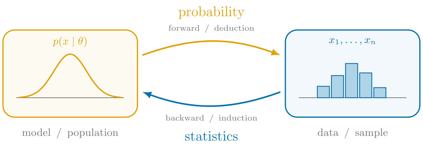
Once a distribution like $p(w|\mathbf{h})$ is inferred from data by research labs, users can use such a distribution in order to generate sentences with an inference loop, namely predicting a distribution over the next token, sampling and appending a token to the history and repeat. Generally speaking, the difference in direction of estimating a distribution from data vs generating data from a distribution is the primary distinction between probability and statistics, although the line as we will soon see gets quite blurry in the same way traditional data and function blurs with software 1.0. This distinction between the two is more broadly known as the difference between analysisanalysis and synthesissynthesissee https://plato.stanford.edu/entries/analytic-synthetic/. Roughly speaking, the former is when you start with something and break it down whereas the latter is when you start with nothing and build it up. Sometimes they are referred to with direction in time: synthesis is the forward direction whereas analysis is the backward.

The users of large language models are generating sentences with conditional distributions over the next word, hence why this most recent wave of methods in software 2.0 is coloquially known as genAIgenerative AI. For instance, in §1.1 From Certain to Uncertain Knowledge we used GPT-2 to produce a conditional distribution $p(w|\text{Hello world, nice to})$ whose next-token prediction capability was in turn used to generate full sentences with the inference loop. In contrast, research engineers at frontier AI labs who are producers of large language modelsOf course, this is falsely dichotomous, for research engineers also use the large language models that they produce. are building the machinery required to produce such estimated distributions $p(w|\mathbf{h})$ from observed samples, namely the entire Internet.

unsupervised learningunsupervised learning supervised learningsupervised learning self-supervised learningself-supervised learning classificationclassification regressionregression

inputsinputs independent variableindependent variable predictorspredictors featuresfeatures

outputsoutputs dependent variabledependent variable responsesresponses targetstargets

two cultures of statisticstwo cultures of statistics

Warning

(todo, also add the two culture parsing/interpretation of the term.) Inference is an overloaded term, and hence ambiguous without context! In generative AI the term inference refers to the forward process of evaluating a population’s distribution $p(w|\mathbf{h})$ in order to generate samples via prediction. In classical statistics the term inference refers to the backward process of inferring a population’s distribution from observed samples (todo estimation and hypothesis testing). Unfortunately terminology and jargon is just like syntax with programming languages! You will need to adjust the meaning of symbols depending on the context, which to foreshadow is precisely what the attention mechanism behind GPT-2’s transformer architecture ends up achieving.

1.2.3 Non-Parametric Histogram with Markov Assumption

So how do we recover the distribution $p(w|\mathbf{h})?$ Rather than strive for perfection, we can achieve the good by introducing some biasbias, known as the markov assumptionMarkov assumption.

• sitll intractable estimate full conditionals by counting relative frequencies of truncated conditional (markov assumption)
  • relative frequency is the MLE estimate
• global vs local distinction. distribution over sentences vs words

a bigram character-level language model adapted from karpathy

dataset = open('./examples/data/names.txt', 'r').read().splitlines()
N = len(dataset)

print("--- TRAINING (counting p(w|h) with python dict ---")
# Histogram (counting frequencies) is the most precise model for training set. it *is* the training set. but it generalizes poorly.
counts_dict = {}
for di in dataset:
  di_normalized = ['<S>'] + list(di) + ['<E>']
  for h,w in zip(di_normalized, di_normalized[1:]): # in the case of bigrams h is a single character, so we can simply zip two strings to get a pair of characters
    # print(h, w)
    counts_dict[(h,w)] = counts_dict.get((h,w), 0) + 1
sorted_counts_dict = sorted(counts_dict.items(), key = lambda x: -x[1])
print("2D (w,h) histogram using python's dict:\n", sorted_counts_dict)


print("--- TRAINING (counting p(w|h) with numpy ndarray (NxN) ---")
# We will now construct the same 2d histogram, but with numpy's ndarray instead of python's dict
# Because numpy's ndarray uses numerical indices to index into, we need to create a dict[str,int]
# so that when we loop over (w,h) pairs within a word we can update the count at the correct location
import numpy as np
vocab = sorted(list(set(''.join(dataset)))) # construct vocab
c2i = {c:i+1 for i,c in enumerate(vocab)}                      # construct map<char,ord>
c2i['.'] = 0                                                                            # with . as the start token and end token, to remove counting freq of (<E>*) and (*<S>) which are all 0
V = len(c2i)                                                                   # evaluate the vocab len V
C_VV = np.zeros((V,V), dtype=np.int32)            # and use V to construct C_VV

# Now we can proceed
for di in dataset:
  di_normalized = ['.'] + list(di) + ['.']
  for h,w in zip(di_normalized, di_normalized[1:]):
    print(h,w)
    h_index, w_index = c2i[h], c2i[w]                                         # use map<char, ord> to lookup the coordinate index needed for C_VV
    C_VV[h_index, w_index] += 1                                                         # update C_VV
print("2D (xt,xt-1) histogram using numpy dict:\n", C_VV)

# normalize counts C_VV to probs P_VV
C_VVf32 = (C_VV+1).astype(np.float32)             # inductive bias (locally smooth)
s_V1 = C_VVf32.sum(axis=1,keepdims=True)                # reduce along axis=1 because we want p(y|x) not p(x|y)
P_VV = C_VVf32 / s_V1                                                                   # (V, V) / (V, 1) broadcasts

# for P_VV, the elements are the counts of bigrams (h,w) accessed by indexing with ord(h) at axis=0 and ord(w) at axis=1
# now, since numpy's ndarray's are row major order, axis=0 gets printed vertically from up to down while axis=1 gets printed horizontally from left to right
i2c = {i:c for c,i in c2i.items()}  # invert map<char, ord> to map<ord, char> because looping with enumerate provides access to indices
header = '    ' + ' '.join(f'{i2c[y_index]:>4}' for y_index in range(V))
print("2D (ord, ord) histogram using numpy ndarray")
print(header)
for w_index, row in enumerate(C_VV+1):
  h = f'{i2c[w_index]:>4}'
  print(h, ' '.join(f'{count:>4}' for count in row))



print("\n\n--- INFERENCE (GENERATING a name by 1. evaluating p(W=w|H=h), appending, and repeating ---")
rng = np.random.default_rng(1337)
sample_count = 10

for _ in range(sample_count):
  h, h_index = [], 0
  while True:
    # 1. evaluate p(W=w|h)
    pWcondH_V = P_VV[h_index].squeeze()

    # 2. sampling
    h_index = rng.choice(len(pWcondH_V), size=1, replace=True, p=pWcondH_V)
    sample_char = i2c[h_index.item()]

    # 3. appending the sample to history
    h.append (sample_char)
    if h_index == 0: break
  print(''.join(h))


loglikelihooddataset,n = 0.0, 0
for di in dataset:
  di_normalized = ['.'] + list(di) + ['.']
  for h,w in zip(di_normalized, di_normalized[1:]):
    w_index, h_index = c2i[h], c2i[w] # use map<char, ord> to lookup the coordinate index needed for P_VV
    pycondx = P_VV[w_index, h_index] # maximize likelihood
    logpycondx = np.log(pycondx)     # maximize loglikelihood

    loglikelihooddataset += logpycondx
    n += 1
    # print(f'{x_char}{y_char}: {pycondx:.4f} {logpycondx:.4f}')



nlldataset = -loglikelihooddataset   # minimize -loglikelihood
avgnlldataset = nlldataset / n       # minimize -1/n loglikelihood
print(f'{loglikelihooddataset=}')
print(f'{nlldataset=}')
print(f'{avgnlldataset=}')

1.2.4 Loss Function with

1.2.5 Evaluation with Perplexity

1.3 Lagniappe: Intelligence as Compression

$\hookleftarrow$ Table of Contents

• information
• entropy

1.4 Categorical Parameterization with Logistic Regression

$\hookleftarrow$ Table of Contents

1.4.1 Architecture with Single Layer Network

1.4.2 Loss Function with Cross Entropy Loss

1.4.3 Optimization with Gradient Descent

1.4.4 Inference, Decision, and Discriminants

discriminant functiondiscriminat function generative modelgenerative model discriminative modeldiscriminative model

• def of conditional
• product rule: joint can evaluated with the chaining of conditionals
• bayes rule: posterior is prior*likelihood over the marginal (what’s the main purpose of this chapter?) (predictive model vs discriminative model vs generative model?)

So how do we recover the distribution $p(w|\mathbf{h})?$ While we know definitionally a probability is a number between 0 and 1 and a distribution is a list of such numbers that normalize to 1, let us consult the definition of a conditional probability. First, let us modify our notation, unravelling the history vector $\mathbf{h}$ into individual components $w_1,w_2,\dots ,w_t$ so that $p(w_{t+1}|w_1,w_2,\dots ,w_t)$ denotes the conditional probability of t+1’th word given the previous t words. Keep in mind that $p(w_1,w_2)=p(w_2,w_1)$, and more generally for any permutation of $w_1,w_2,\dots ,w_t$, since each random variable $W_i=w_i$ models the event that the ith position of a sentence length $t$ takes on certain value. That is, order is modeled into our random variables, and so joint probabilities remain commutative (todo. big jump here).

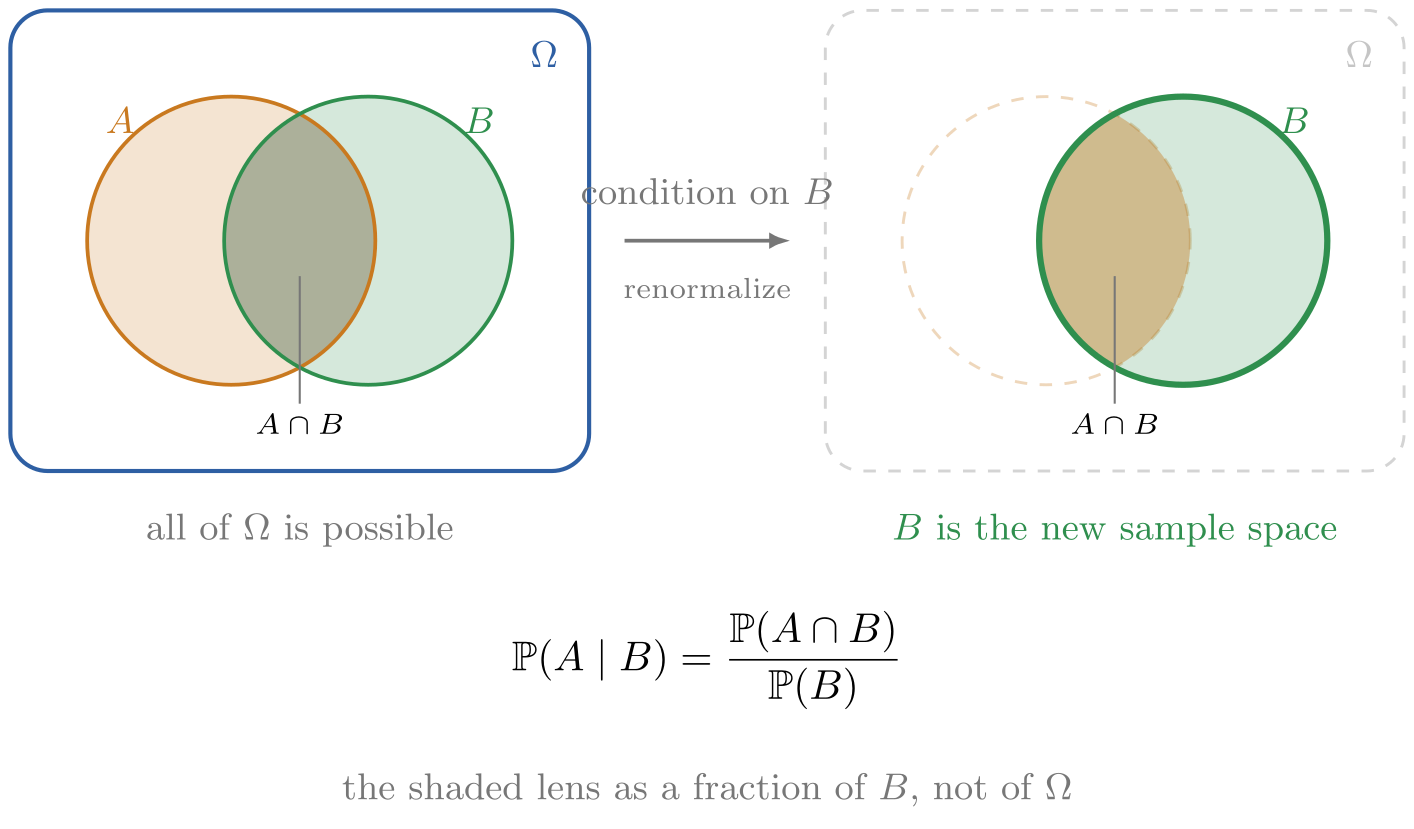
Then, definitionally speaking, the conditional distributionconditional distribution is defined as the ratio between the joint distributionjoint distribution of the two random variables (the one of interest, namely the next word, and the one that is being conditioned on, namely the previous words) and the distribution of the random variable that is being conditioned on, which corresponds with our intuition that the Venn diagram suggests:

• todo: bayes rulebayes rule
• todo: connect bayes rule over language to bayes rules over functions

$$\begin{array}{rl}p(w_{t+1}|w_1,w_2,\dots ,w_t)& \stackrel{△}{=}\frac{p(w_{t+1},w_1,w_2,\dots ,w_t)}{p(w_1,w_2,\dots ,w_t)}\end{array}$$

and rearrange the identity for the joint, we have that

$$\begin{array}{r}p(w_{t+1},w_1,w_2,\dots ,w_t)=p(w_1,w_2,\dots ,w_t)p(w_{t+1}|w_1,w_2,\dots ,w_t)\end{array}$$

known as the product ruleproduct rule, and reads that the probability of a t-length sentence is equivalent to the probability of the first t words multiplied by the probability of t+1’th word occuring given the first t words occured. The product rule is the probability of logical AND alongside the sum rule for the probability of logical OR. The product rule is also referred to as the chain rulechain rule given that we are chaining probabilities together, and is the primary mechanism of generation within a large language model’s inference loop. Morever, the fact that these distributions $p(\circ )$ are functions $p:\mathbb{N}\to [0,1]$ means that the division and multiplication in numpy are implemented via element-wise operationelement-wise operators.

[!QUESTION] Given that you know $p(w|\mathbf{h})\in {\mathbb{R}}^{|V|}$, what do you expect the types of the two distributions $p(w_{t+1},w_1,w_2,\dots ,w_t)$ and $p(w_1,w_2,\dots ,w_t)$ and the shapes of their corresponding np.ndarray’s to be? Prompt a language model to implement what you think. Pause, think and prompt!

Click to reveal answer

The type of $p(w_{t+1},w_1,w_2,\dots ,w_t)$ is some function $p:\mathbb{N}\to {\mathbb{R}}^{V\times V\times \cdots \times V}$, or some np.ndarray with .shape (V, V, V, V, V).

If we had access to such distributions,

import numpy as np
history_VVVV = np.array_with_shape((V, V, V, V, V, V)) # t=4, i.e "Hello world, nice to"
joint_VVVVV = np.array_with_shape((V, V, V, V, V, V)) # t=5, i.e p("Hello world, nice to") AND p("you") 
conditional = joint_VVVVV / history_VVVV # broadcast

1.4.3 Evaluation with Bias Variance Tradeoff

1.5 Quantitative Redux with Linear Regression

$\hookleftarrow$ Table of Contents

• why squared error loss from artem

Similarly to learning distributions $X$ from data, learning functions $f:\mathcal{X}\to \mathcal{Y}$ from data roughly follows the three step process of selecting a model for the task $T$, a performance measure $P$, and optimizing such measure on experience $E$. Let’s take a look at the linearly modeling regression with squared error loss, a problem which straddles tools from all three languages of probability theory, linear algebra, and calculus.

For the task of house price prediction, the input space $\mathcal{X}={\mathbb{R}}^d$ is the size in square feet, and the output space $\mathcal{Y}=\mathbb{R}$ is the price, meaning that the function which needs to be recovered has the type of $f:{\mathbb{R}}^d\to \mathbb{R}$. An assumption about the structure of the data needs to be made, referred to as the inductive bias. The simplest assumption to make is to assume that there exists some linear relationship between the data $\mathbf{x}$ and parameters $\mathbf{w}$ so that $f$ ends up being modeled as an inner product plus bias, parameterized as $f(\mathbf{x};\mathbf{w},b)$: $$\begin{array}{rl}f& :{\mathbb{R}}^d\to \mathbb{R}\\ f(\mathbf{x};\mathbf{w},b)& :=({\mathbf{w}}_1{\mathbf{x}}_1+{\mathbf{w}}_2{\mathbf{x}}_2+\cdots +{\mathbf{w}}_n{\mathbf{x}}_n)+b\\ & =(\sum _{i=1}^d{\mathbf{w}}_i{\mathbf{x}}_i)+b\\ & ={\mathbf{w}}^{\top }\mathbf{x}+b\end{array}$$

One small adjustment we can make to $f$ is to fold the final bias term $b$ into the vector $\mathbf{w}$ as ${\mathbf{w}}_1$, increasing the total dimensionality so that $\mathbf{w}\in {\mathbb{R}}^{d+1}$, and adjusting $\mathbf{x}$ accordingly so that ${\mathbf{x}}_1:=1$ and $\mathbf{x}\in {\mathbb{R}}^{d+1}$. Then, the equation of our line with bias is simply parameterized as $f(\mathbf{x};\mathbf{w})$ $$\begin{array}{rl}f& :{\mathbb{R}}^{d+1}\to \mathbb{R}\\ f(\mathbf{x};\mathbf{w})& :={\mathbf{w}}^{\top }\mathbf{x}\end{array}$$

Semantically speaking, each property of the input house ${\mathbf{x}}_i\in {\mathbb{R}}^d$ is weighted by some weight ${\mathbf{w}}_i$, adjusted accordingly during the learning process so that it accurately reflects the property’s influence on the output price $y\in \mathbb{R}$ when evaluating a prediction $\hat{y}$. We can evaluate $f$ on all ${\mathbf{x}}^{(i)}\in \mathcal{D}$ with a randomly intialized $\mathbf{w}$ to ensure we’ve wired everything up correctly.

However, while specifying the equation of the linear regression model on paper screen and subsequently evaluating the computation manually might have been sufficient for pre-computational mathematicians such as Gauss and Legendre, the discipline of statistical learning is entirely predicated on computational methods. Let’s continue to use PyTorch’s core n-dimensional array datastructure with torch.Tensor, this time modeling a function $f:\mathcal{X}\to \mathcal{Y}$ rather than some distribution $X$:

(todo: maybe change example to closure following torch.nn)

{{#include ../../teeny/examples/2.2-regression.py:1:4}}

in which we can update the names of our torch.Tensor variables with the ranks of their vector spacesReferred to as Shape Suffixes, described by Noam Shazeer, an engineer from Google to clarify what dimensions these operations are evaluated on:

{{#include ../../teeny/examples/2.2-regression.py:5:8}}

and finally, actually enforce them via runtime typechecking with the jaxtyping package (try swapping the return statements below to trigger a type error with the return type):

{{#include ../../teeny/examples/2.2-regression.py:9:19}}

Let’s now sanity-check that f_typechecked is wired up correctly by evaluating it on all ${\mathbf{x}}^{(i)}\in \mathcal{D}$ with random parameter w_D. (todo: use actual housing data)

{{#include ../../teeny/examples/2.2-regression.py:29:41}}

random weight vector: tensor([-0.3343,  0.0768,  2.7828, -0.1331])
expected: $500000.0, actual: $-492.46
expected: $800000.0, actual: $-690.89
expected: $250000.0, actual: $-258.08

Clearly, these outputs are unintelligible, and will only become intelligible with a “good” choice of parameter $\mathbf{w}$. Before we find such a parameter, let’s make one more modification to our function $f$ to increase it’s performance. Rather then evaluating f_typechecked on every input xi_D in the dataset zip(X_ND,Y_N) sequentially with a loop, we can evaluate all outputs with a single matrix-vector multiplication by updating $f$’s function definition to the following

$$\begin{array}{rl}{f}_{\text{batched}}& :{\mathbb{R}}^{n\times d}\to {\mathbb{R}}^n\\ f_{\text{batched}}(\mathbf{X};\mathbf{w})& :=\mathbf{Xw}\\ & =\left[\begin{array}{c}{\mathbf{x}}_1^{\top }\mathbf{w}\\ {\mathbf{x}}_2^{\top }\mathbf{w}\\ ⋮\\ {\mathbf{x}}_n^{\top }\mathbf{w}\end{array}\right]\end{array}$$

and the corresponding PyTorch updated to

{{#include ../../teeny/examples/2.2-regression.py:21:27}}

Now that we’ve selected our model for the task $T$, we can proceed with selecting our performance measure $P$ which the learner will improve on with experience $E$.

After the inductive bias on the family of functions has been made, the learning algorithm must find the function $\hat{f}$ with a good fit. Since artificial learning algorithms don’t have visual cortex like biological humans[], the notion of “good fit” needs to defined in a systematic fashion. This is done by selecting the parameter $\theta \in {\mathbb{R}}^m$ which maximizes the likelihood of the data $p(d;\theta )$. Returning to the linear regression inductive bias we’ve selected to model the house price data, we assume there exists noise ${ϵ}^{(i)}$ in both our model (epistemic uncertainty) and data (aleatoric uncertainty), so that $y^{(i)}={\theta }^{\top }{\mathbf{x}}^{(i)}+{ϵ}^i$ where ${ϵ}^{(i)}\sim \mathcal{N}(\mu ,{\sigma }^2)$

prices $y^i$ are normally distributed conditioned on seeing the features ${\mathbf{x}}^i$ with the mean being the equation of the line ${\theta }^{\top }{\mathbf{x}}^{(i)}$ where $y^{(i)}|{\mathbf{x}}^{(i)}\sim \mathcal{N}(\mu ={\theta }^{\top }{\mathbf{x}}^{(i)},{\sigma }^2)$, then we have that

$$\begin{array}{rl}p(y^{(i)}|{\mathbf{x}}^{(i)};\theta )& =\mathcal{N}({\theta }^{\top }{\mathbf{x}}^{(i)},{\sigma }^2)\\ & =\frac{1}{\sqrt{2\pi {\sigma }^2}}\exp \left(-\frac{(y^{(i)}-{\theta }^{\top }{\mathbf{x}}^{(i)}{)}^2}{2{\sigma }^2}\right)\end{array}$$

TODO: generate prose/exposition by repaging lecture/text in ram

Returning to the linear regression model, we can solve this optimization with a direct method using normal equations. QR factorization, or SVD.

def fhatbatched(X_n: np.ndarray, m: float, b: float) -> np.ndarray: return X_n*m+b

if __name__ == "__main__":
  X, Y = np.array([1500, 2100, 800]), np.array([500000, 800000, 250000]) #  data

  X_b = np.column_stack((np.ones_like(X), X))              # [1, x]
  bhat, mhat = np.linalg.solve(X_b.T @ X_b, X_b.T @ Y)   # w = [b, m]

  yhats = fhatbatched(X, mhat, bhat) # yhat
  for y, yhat in zip(Y, yhats):
    print(f"expected: ${y:.0f}, actual: ${yhat:.2f}")

To summarize, we have selected and computed

1. an inductive bias with the family of linear functions $f(\mathbf{X};\theta ):=\mathbf{X}@\theta$
2. an inductive principle with the least squared loss $\mathcal{L}(\theta ):={\sum }_{i=0}^n(y^{(i)}-\mathbf{X}@\theta {)}^2$
3. the parameters which minimze the empirical risk, denoted as $(\hat{\theta })=\mathrm{argmin}\mathcal{L}(\theta )$

Together, the inductive bias describes the relationship between the input and output spaces, the inductive principle is the loss function that measures prediction accuracy, and the minimization of the empirical risk finds the parameters for the best predictor.

1.5 Bias Variance Tradeoff

1.6 Summary

$\hookleftarrow$ Table of Contents

1.7 Further Reading

$\hookleftarrow$ Table of Contents

The primary texts consulted in the writing of this chapter were (Jurafsky and Martin 2026), (Eisenstein 2018), (Manning 2001), and (Cotterell 2024) for statistical natural language processing; (Bishop 2006) (Hastie, Tibshirani, and Friedman 2009), (Murphy 2022), (Mohri et al., 2018), and (Bach 2025), for machine learning more generally.

1.8 Problems

$\hookleftarrow$ Table of Contents

Intermezzo One: The Language of Probability Theory and Linear Algebra

$\hookleftarrow$ Table of Contents

As you now know from §1. Sequence Learning, language models are next token predictors. Whether these language models are bigram models, logistic regression models, or the GPT-2 like neural nets that we will see in Part II. Deep Neural Networks, they are all functions that produce an output distribution over the next word given some input sentence as the history. That is, they are functions of type $f:{\Sigma }^{\ast }\to {\Delta }^{|\Sigma |}$ Before we dive into the internals of teenygrad itself in §2. The Tensor and implement our own framework capable of training the bigram and logistic regression models, we will formally characterize our language model implementations from §1 using the language of calculus from high school, as well as probability and linear algebra which we will formally introduce now. The one text which was heavily consulted over others was Formal Aspects to Language Modelling (Cotterell et al., 2024). For more on formalization, please consult §A. From Problems to Proof.

I.1 Probability Spaces

$\hookleftarrow$ Table of Contents (Intermezzo One)

Informally speaking, you intuitively understand the notion of a probability and a probability distribution. That is, a probability is a number between 0 and 1 that represents the chance, likelihood, or belief of some event happening, and a distribution is a list of such numbers. Probability distributions come from the concept of probability spaces, so before defining the former we must define the latter, which are measures of the size of sets.

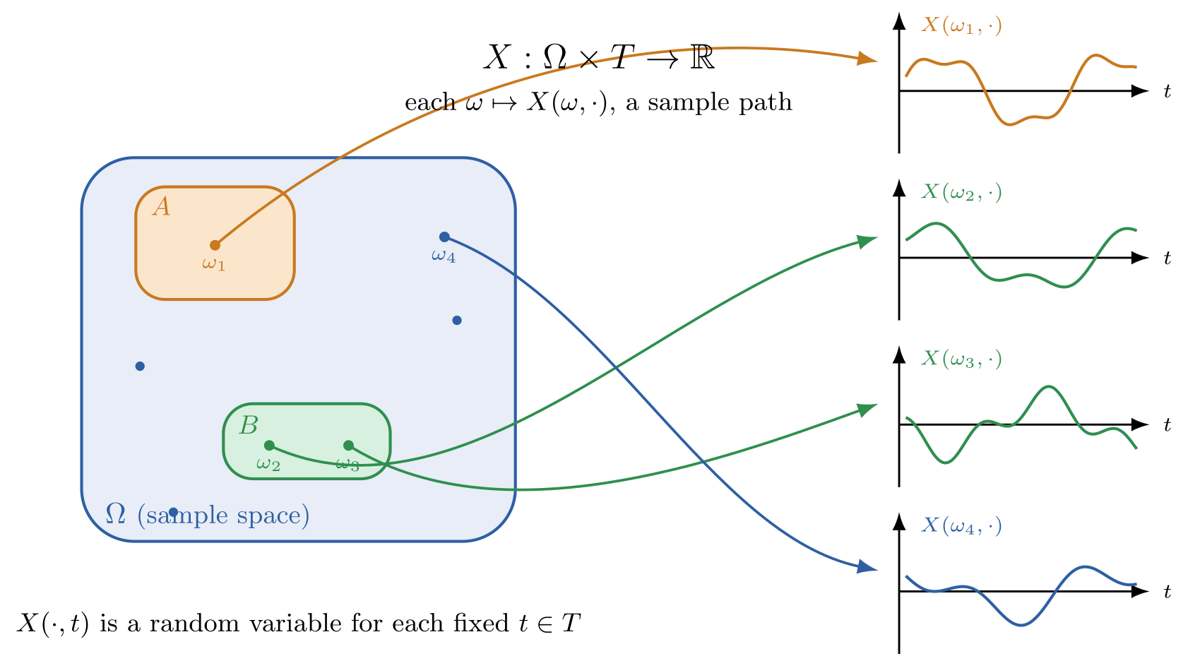
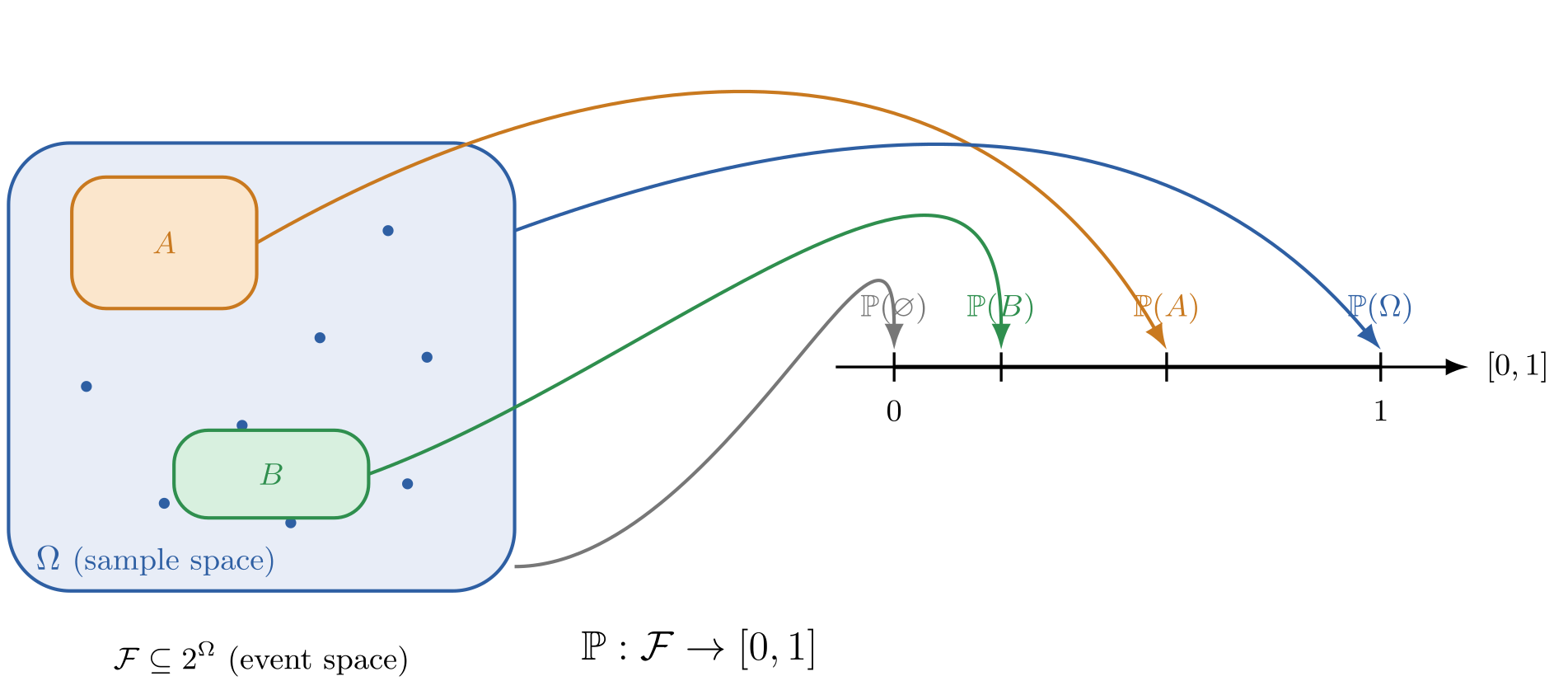Figure I.1 is comprised of three components. Namely, the blue box and it’s blue dots, the colored boxes, and the mapping from the colored boxes to the $[0,1]$ number line

1. the sample space $\Omega$: the set of all possible outcomes in an experiment
2. the event space $\mathcal{F}$: the set of all subsets in the sample space
3. probability law $\mathbb{P}$: a mapping from the event space to a number between 0 and 1

Conceptually speaking, the language models we’ve seen in §1. Sequence Learning such as GPT-2, the bigram model, and the logistic regression model which have type $f:{\Sigma }^{\ast }\to {\Delta }^{|\Sigma |}$ produce (on a single evaluation) concrete probability distributions with np.ndarray that come from mathematically abstract probability spaces $(\Omega ,\mathcal{F},\mathbb{P})$ where the sample space $\Omega$ is the set of words in their vocabulary, and their belief in a word occuring is represented by probability law $\mathbb{P}$ defined on event space $\mathcal{F}$.

Caution

Probability spaces are usually NOT implemented with code. For instance, GPT-2, bigram models, and logistic regression models do NOT instantiate and return Python set()s for the sample space $\Omega$, the event space $\mathcal{F}$, nor define some function def probability_law(event_space: set) -> float for $\mathbb{P}$. They return a probability distributions, which we define in §I.2 Random Variables and their Distributions. Rather, the purpose of probability spaces as a mathematical definition is conceptual clarity with general definitionsDefining concepts without commiting to internal structure allows for a much broader class of objects to be considered. This is very much like type polymorphism (generics, traits, type classes), except the generality of mathematical concepts are usually “more” general than those that might be implemented with type polymorphism. For instance, this abstract definition of a probability space is generalized to cover any random experiment we’d like to model, from rolling dice, to generating language. However it’s quite unusual to have a program need to progam both. and rigorous results with theorems.

Let us now precisely define each component of a probability space $(\Omega ,\mathcal{F},\mathbb{P})$, starting with the sample space $\Omega$.

So conceptually speaking, language models like GPT2, the bigram model, and the logistic regression model of type $f:{\Sigma }^{\ast }\to {\Delta }^{|\Sigma |}$ which produce concrete distributions with np.ndarray on a single evaluation come from mathematically abstract probability spaces $(\Omega ,\mathcal{F},\mathbb{P})$ where the sample space $\Omega$ is the set of words in their vocabulary, and their belief in a word occuring is represented by probability law $\mathbb{P}$ defined on event space $\mathcal{F}$.

Important

Notice how we have NOT said anything about multiple evaluations of a language model’s output distribution (and probability space) over words to generate a complete sentence (in the probablity space of sentences). We will see how they relate soon.

TODO: something to say here about event spaces? cardinality of them?

[!QUESTION] Why is the probability law $\mathbb{P}$ defined as a function on the event space $\mathcal{F}$ rather than the sample space $\Omega$? Pause, think! Hint: Would something bad happen if we did such a thing?

$$\begin{array}{rlrl}\mathbb{P}(\{\text{banana},\text{bongo}\})& =\mathbb{P}(\{\text{banana}\}\cup \{\text{bongo}\})& & \\ & =\mathbb{P}(\{\text{banana}\})+\mathbb{P}(\{\text{bongo}\})& & \text{[by additivity]}\\ & =0.1+0.2& & \\ & =0.3& & \end{array}$$

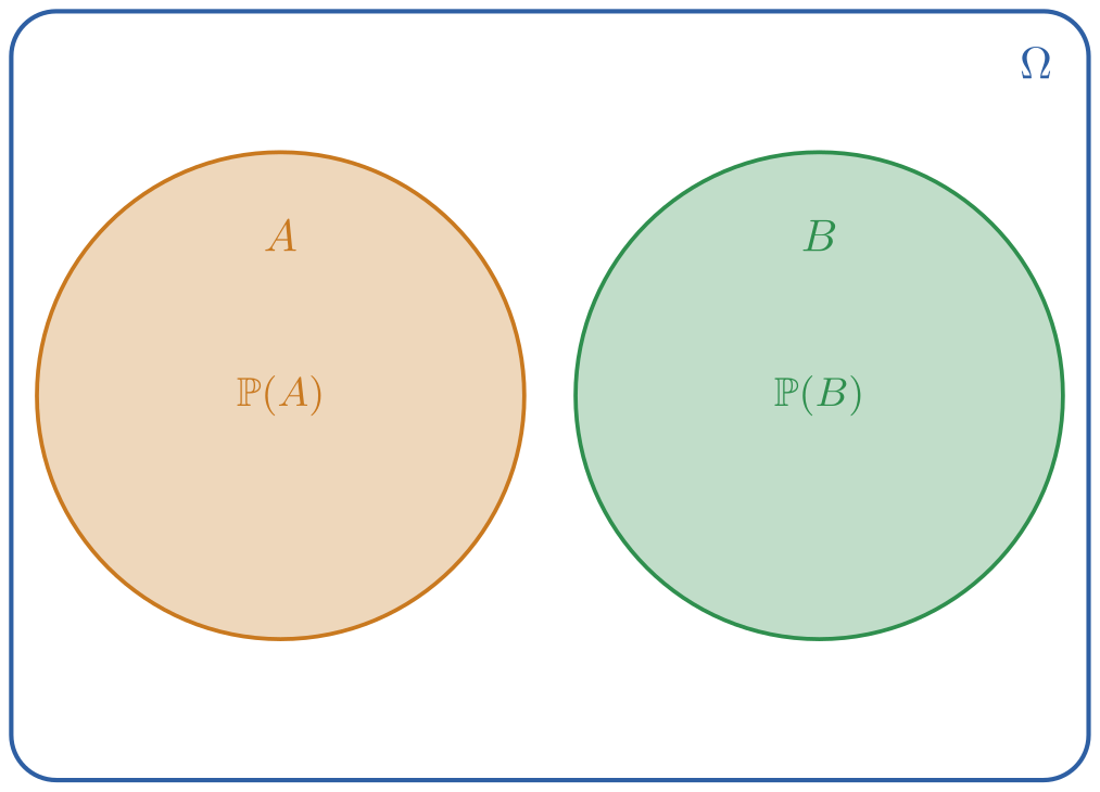
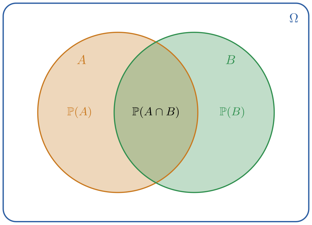
However the event $C$ which contains all foobarbaz is composed of overlapping events (corresponding to the right figure above), so the axiom of addivitiy does not apply. We can evaluate the union of non-disjoint (overlapping) events with the following corollary, known as the sum rulesum rule:

$$\mathbb{P}(A\cup B)=\mathbb{P}(A)+\mathbb{P}(B)-\mathbb{P}(A\cap B)$$

We have now sharpened our intuitive notion of chance, belief, and probability by formally defining them as the measure of the size of sets. These sets have a home, and the measure has a domain, namely the sample space $\Omega$ and the event space $\mathcal{F}$ and together with the probability law $\mathbb{P}$, comprise the definition of a probability space $(\Omega ,\mathcal{F},\mathbb{P})$, albeit abstractly so. Let us now connnect this mathematically abstract space to the more concrete probability distributions we used in §1. Sequence Learning.

I.2 Random Variables and their Distributions

$\hookleftarrow$ Table of Contents (Intermezzo One)

Probability distributions are the practical and concrete np.ndarrays we used throughout §1. Sequence Learning when implementing the bigram and logistic regression language models. So how do these connect to the abstract concept of probability spaces just defined? The answer is with random variables and their probability mass functions, which are functions that map outcomes to states, and from states to probabilities.

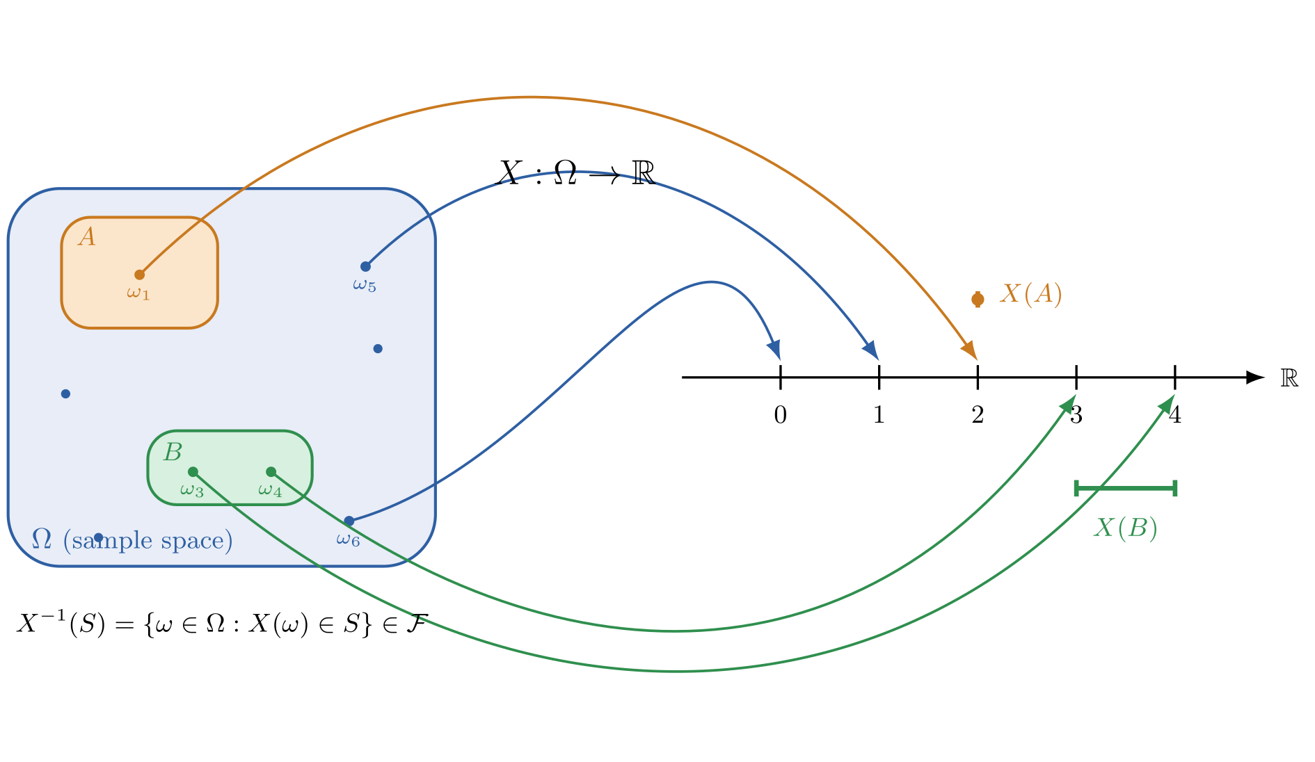
Figure I.2

(todo modify picture or include another picture to show distribution (probality assignment of variable taking on state))

Figure I.2 shows the same sample space $\Omega$ and event space $\mathcal{F}$ from §I.1 Probability Spaces, but rather than evaluate probabilities with the probability law $\mathbb{P}:\mathcal{F}\to [0,1]$ by mapping events to the [0,1] number line (displayed in Figure I.1), we create one level of indirection with

• a random variable $X:\Omega \to \mathbb{R}$ mapping outcomes in the sample space to states on the real number line and then defining
• a probability mass function $p_X(x):\mathbb{R}\to [0,1]$ mapping states to their probabilities.

So, starting with a sample space, you have to map outcomes to their state space with a random variable before you can evaluate their probabilities with a probability mass function, rather than evaluate them directly with a probability law. In other words, the two types are not equivalent $p_X(x):\mathbb{R}\to [0,1]\ne \mathbb{P}:\mathcal{F}\to [0,1]$. For example, recall from §1.1 From Certain to Uncertain Knowledge GPT-2’s np.ndarray output probs when passed the input string "Hello world, nice to":

import numpy as np

# GPT-2's output distribution when passed input "Hello world, nice to"
# Showing top 10 most likely words out of 50257.
tokens = [" see", " meet", " hear", " have", " be", " know", " you", " talk", " say", " get"]
probs = np.array([0.3169, 0.1268, 0.1246, 0.1046, 0.0471, 0.0352, 0.0320, 0.0128, 0.0114, 0.0067])
for i in np.argsort(-probs):
    print(f"{tokens[i]} : {probs[i]:.4f}")

Here, there is a random variable $X:\Omega \to \mathbb{R}$ which maps outcomes from the abstract sample space $\Omega :=\{\text{see},\text{meet},\text{hear},\text{have},\text{be},\text{know},\text{you},\text{talk},\text{say},\text{get}\}$ to concrete states $x$ in state space $\mathbb{R}$. That is,

$$\begin{array}{rl}& X:\Omega \to \mathbb{R}\\ & X(\text{see})\mapsto 0,X(\text{meet})\mapsto 1,X(\text{hear})\mapsto 2,X(\text{have})\mapsto 3,X(\text{be})\mapsto 4,X(\text{know})\mapsto 5\\ & X(\text{you})\mapsto 6,X(\text{talk})\mapsto 7,X(\text{say})\mapsto 8,X(\text{get})\mapsto 9\end{array}$$

But notice the level of indirection with the random variable. All we’ve done is translate from sample space to state space. To obtain actual probabilities, we need to map from the state space $\mathbb{R}$ to probabilities $[0,1]$ with the probability mass function $p_X(x):\mathbb{R}\to [0,1]$. That is,

$$\begin{array}{rl}& p_X:\mathbb{R}\to [0,1]\\ & p(0)\mapsto 0.3169,p(1)\mapsto 0.1268,p(2)\mapsto 0.1246,p(3)\mapsto 0.1046,p(4)\mapsto 0.0471,p(5)\mapsto 0.0352\\ & p(6)\mapsto 0.0320,p(7)\mapsto 0.0128,p(8)\mapsto 0.0114,p(9)\mapsto 0.0067\end{array}$$

In other words, starting from sample space $\Omega$ we compose $X:\Omega \to \mathbb{R}$ with $p_X(x):\mathbb{R}\to [0,1]$ to obtain $p_X\circ X:\Omega \to [0,1]$ such that evaluating $p(X(\omega ))$ results in the probability of outcome $\omega$. (todo. this is wrong?)

But how is the multidimensional array probs with support in ${\mathbb{R}}^{|V|}$ related to the abstract concept of a probability space? You may have noticed that the definition of $p_X$ looks quite similar to that of the probs:

import numpy as np
probs = np.array([0.3169, 0.1268, 0.1246, 0.1046, 0.0471, 0.0352, 0.0320, 0.0128, 0.0114, 0.0067])

This is because an alternative conceptualization of ${\mathbb{R}}^{10}$ is some function $f:\{0,1,2,3,4,5,6,7,8,9\}\to \mathbb{R}$For conveniece sake we do store the outcomes in the tokens array so that we can print them next to their probabilities by looping over states $x\in \mathbb{R}$ with for i in np.argsort(-probs), but it’s important to note that $p_X(x)$ is defined on real numbered states (represented with indices), and not on set-valued events. that has support in ${\mathbb{R}}^{10}$, or more accurately, $\{0,1{\}}^{10}$ With these two views, an alternative conceptualization of ${\mathbb{R}}^{10}$ is some function $f:\{0,1,2,3,4,5,6,7,8,9\}\to \mathbb{R}$

• todo: rvs map from one measurable space to another. we happen to like $\mathbb{R}$

On a single evaluation language models produce such probability mass functions defined on a state space which are mapped over from an abstract sample space via random variable. In practice, we forget about the concepts of sample spaces and random variables, simply slugging around probability mass functions with np.ndarrays that have support in n-dimensional Euclidean space, where n is the size of sample space. In other words, we keep two as conceptual mathematical definitions without implementing them with code.

At this point, you may be wondering what is the point of the random variable’s indirection? … Now that you understand the notion of random variables and probability mass functions intuitively, let’s formally define them as concepts:

somehow motivate global view

The intuition is very simple: every language model can be locally normalized. The precise formulation however, is not. proof with prefix probabilities

however the converse direction is not a trivial result to establish examples

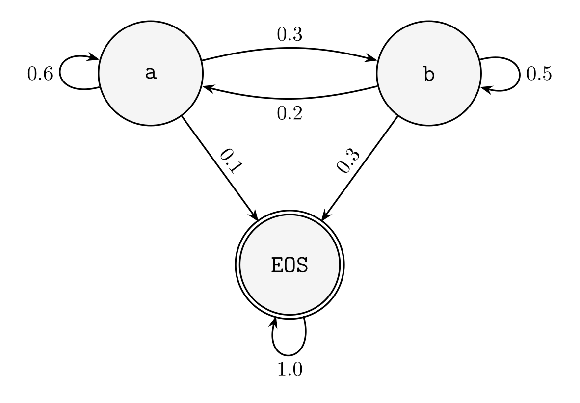
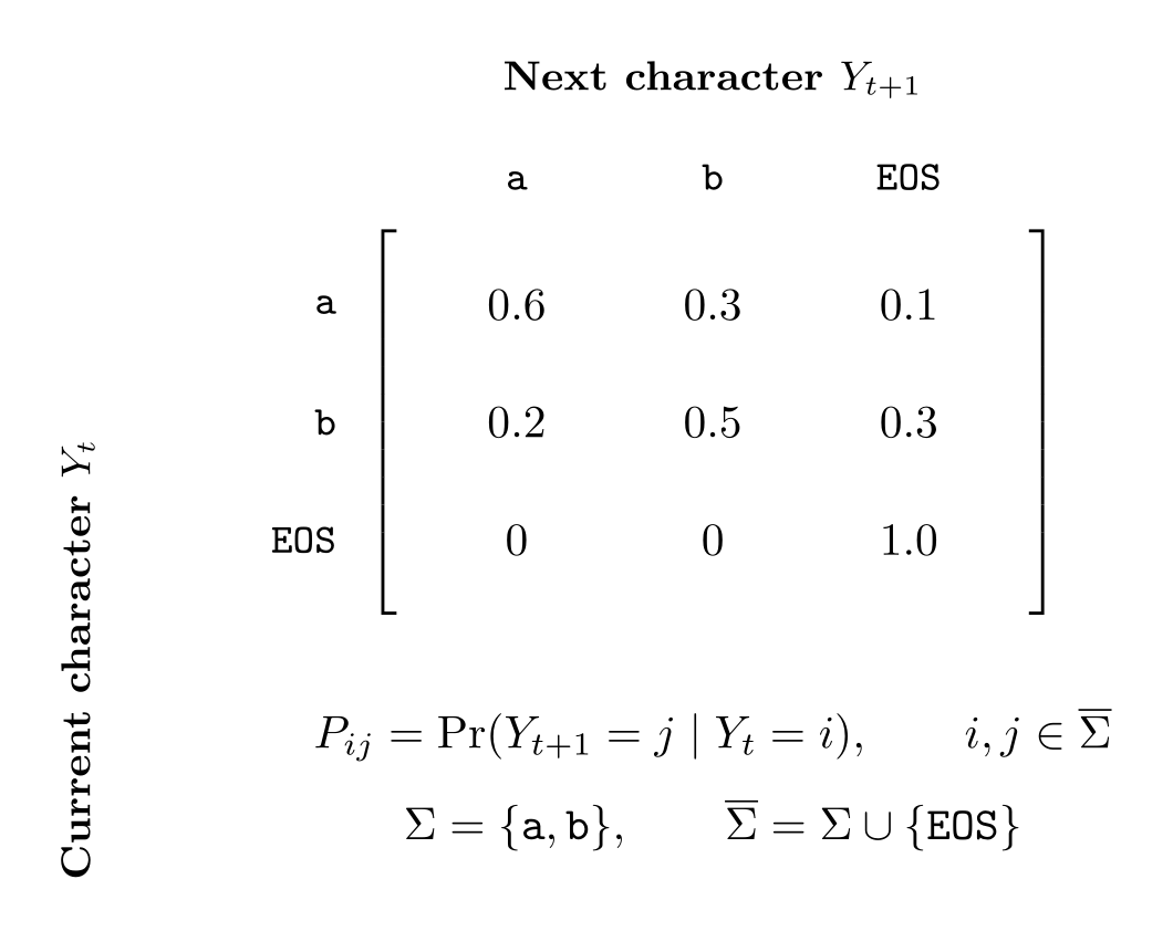
• 2 state model (markov chain), non-tight
• 2 state model (markov chain), tight (absorbs)

I.3 Probabilities of Sums, Products, Conditionals

I.4 Random Processes and their Kernels

$\hookleftarrow$ Table of Contents (Intermezzo One)

I.5 Measurable Spaces

I.6 Vector Spaces

$\hookleftarrow$ Table of Contents (Intermezzo One)

I.7 Further Reading

The primary texts consulted in the writing of this chapter were (Bertsekas and Tsitsiklis 2008), (Chan 2021), (Wasserman 2004), and (Durrett (2019) for probability theory; (Strang 2026), (Strang 2019), and (Axler 2026) for linear algebra; (Boyd and Vandenberghe 2004) and (Kochenderfer and Wheeler 2019) for optimization.

2. From IPL’s Array to APL’s Multidimensional Array

$\hookleftarrow$ Table of Contents

2.1 From Virtual to Physical Machines (and Shapes)

$\hookleftarrow$ Table of Contents

• justify native for eager performance
• pyo3 https://github.com/j4orz/ateenysitp/blob/master/ARCHITECTURE.md#level-1-teenygrads-build-configuration-and-development-environment
• native components using cpython as encapsulation boundary
• freethreaded python eliminates multithreading problem

/// SGEMM with the classic BLAS signature (row-major, no transposes):
/// C = alpha * A * B + beta * C
fn sgemm(
  m: usize, n: usize, k: usize,
  alpha: f32, a: &[f32], lda: usize,
  b: &[f32], ldb: usize,
  beta: f32, c: &mut [f32], ldc: usize) {
  assert!(m > 0 && n > 0 && k > 0, "mat dims must be non-zero");
  assert!(lda >= k && a.len() >= m * lda);
  assert!(ldb >= n && b.len() >= k * ldb);
  assert!(ldc >= n && c.len() >= m * ldc);

  for i in 0..m {
    for j in 0..n {
      let mut acc = 0.0f32;
      for p in 0..k { acc += a[i * lda + p] * b[p * ldb + j]; }
      let idx = i * ldc + j;
      c[idx] = alpha * acc + beta * c[idx];
    }
  }
}

fn main() {
  use std::time::Instant;

  for &n in &[16usize, 32, 64, 128, 256] {
    let (m, k) = (n, n);
    let (a, b, mut c) = (vec![1.0f32; m * k], vec![1.0f32; k * n], vec![0.0f32; m * n]);

    let t0 = Instant::now();
    sgemm(m, n, k, 1.0, &a, k, &b, n, 0.0, &mut c, n);
    let secs = t0.elapsed().as_secs_f64().max(std::f64::MIN_POSITIVE);
    let gflop = 2.0 * (m as f64) * (n as f64) * (k as f64) / 1e9;
    let gflops = gflop / secs;

    println!("m=n=k={n:4} | {:7.3} ms | {:6.2} GFLOP/s", secs * 1e3, gflops);
  }
}

2.2 Accelerating the Communication of Hierarchies

Loop Reordering, Register and Cache Blocking

$\hookleftarrow$ Table of Contents

2.3 Accelerating the Computation of Pipelines

$\hookleftarrow$ Table of Contents

Instruction Level Parallelism via Loop Unrolling

2.4 From Abstract to Numerical Linear Algebra

2.6 Summary

One quick way to summarize the milestones in high performance computing, compilers and architecture is to list the Turing Award winners: Alan Perlis (1966) for his influence on advanced programming techniques and compiler construction, including his role in designing ALGOL and establishing the discipline of programming languages as a field; John Backus (1977) for designing FORTRAN — the first high-level language to achieve widespread practical adoption — and formalizing language syntax through Backus-Naur Form; Tony Hoare (1980) for axiomatic semantics, giving programmers a formal logical framework for reasoning about program correctness; Niklaus Wirth (1984) for designing a sequence of clean, teachable languages — EULER, ALGOL-W, Pascal, and Modula — that shaped how programming languages are structured and implemented; John Cocke (1987) for pioneering optimizing compilers and the Reduced Instruction Set Computer (RISC) architecture, showing that simpler instruction sets allow faster hardware; William Kahan (1989) for fundamental contributions to numerical analysis, most consequentially the IEEE 754 floating-point standard that made reliable numerical computation reproducible across hardware; Frederick Brooks (1999) for landmark contributions to computer architecture — most notably the IBM System/360 — and for articulating the enduring lessons of large-scale software engineering; Frances Allen (2006) for foundational contributions to the theory and practice of optimizing compilers, including dataflow analysis and the program dependence graph; John Hennessy and David Patterson (2017) for a systematic, quantitative approach to designing and evaluating computer architectures, whose RISC principles underpin billions of processors and the open RISC-V standard; and Alfred Aho and Jeffrey Ullman (2020) for foundational contributions to programming language theory and compiler construction, most durably codified in the Dragon Book; and finally,Jack Dongarra (2021) for pioneering the numerical libraries — BLAS, LAPACK, and MPI — that became the substrate of high-performance scientific computing and modern deep learning accelerators;

2.7 Further Reading

The primary texts consulted in the writing of this chapter were

2.8 Problems

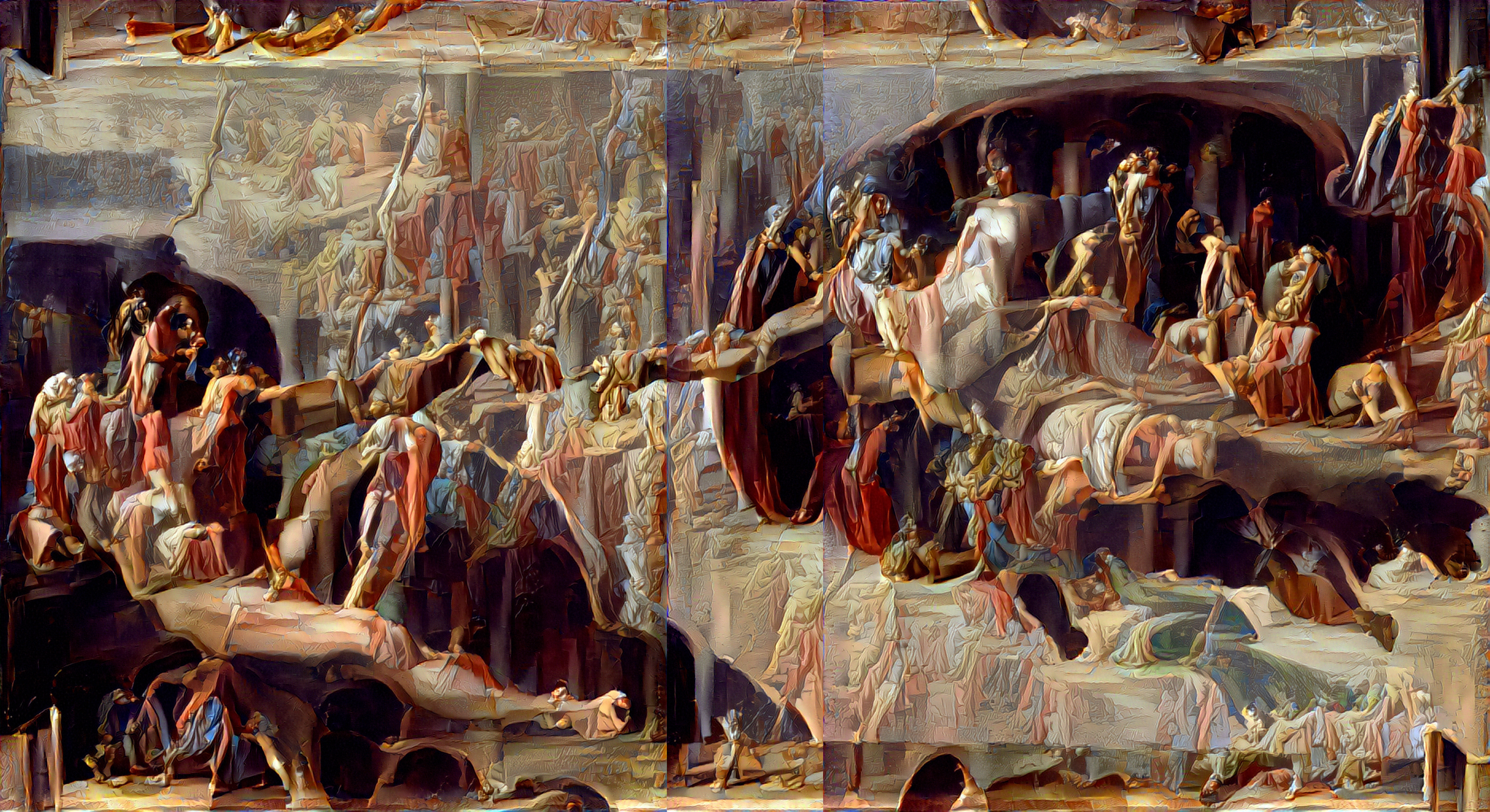The Creation of Adam, Michelangelo 1508-1512.

II. Neural Networks

In part one of The Structure and Intepretation of Tensor Programs you have developed a solid foundation in the mathematical preliminaries and statistical models used throughout the machine learning approach to artificial intelligence. It’s amazing how close you are to of deep learning without you even knowing. By the end of Part II. Neural Networks, we will be one step closer in achieving our quest of building our own ChatGPT by reproducing GPT2Presented in Language Models are Unsupervised Multitask Learners (Raford et al. 2019), following Andrej Karpathy’s nanogpt. But before we get there, there is some more work for us to do.

So in Chapter 4. Learning Sequences via Deep Neural Networks with teenygrad, you will increase the expressivity of the linear models implemented in Part I by non-linearities to get a class of models known as deep neural networks. In order to build ourselves up to nanogpt, we will hold the training goal of learning sequences constant, and incrementally implement more expressive neural networks architectures following the nets in Andrej Karpathy’s makemore, starting from feedforward neural networks (FNNs), to convolutional neural networks (CNNs), to recurrent neural networks (RNNs), and finally, transformer neural networks (GPTs). These various neural network architectures implement different inductive biases, which were all explored during the 2012-2019 time period of what is coloqially known as the age of research.

Then, in Chapter 5. Accelerating Sequence Models on GPU in teenygrad, you will evolve teenygrad from a numerical linear algebra library implemented in Part I to a full blown batteries-included deep learning framework like PyTorch. This means implementing the optimizers for neural networks whose evaluations are accelerated with massively parallel processors and whose gradients are automatically evaluated with an automatic differentiation engine.

After completing part two, you will be ready for Part III. Scaling Networks of the book where we finally achieve our quest of building our own ChatGPT. Part three follows the 2020-2025 time period of what is colloquially as the age of scaling where researchers focused on scaling up the generality of generative pretrained transformers by adding assistant-like behavior in a midtraining phase with reinforcement learning with human feedbackOriginally presented in Introducing ChatGPT (OpenAI 2022), and reproduced by open source in Llama 2: Open Foundation and Fine-Tuned Chat Models (Touvron et al. 2023) and by adding reasoning-like behavior in a posttraining phase with foobarbazOriginally presented in Introducing OpenAI o1 (OpenAI 2024), and reproduced by open source in DeepSeek-R1: Incentivizing Reasoning Capability in LLMs via Reinforcement Learning

II. Neural Networks

4. Learning Sequences from Data with Deep Neural Networks in torch

$\hookleftarrow$ Table of Contents

(todo, some explanation) on learning sequences

4.1 From Supervised to Self-Supervised Learning with Sequences

4.2 Learning Sequences with Linear Models

4.3 From Linear to Non-Linear Learning with Deep Neural Networks

$\hookleftarrow$ Table of Contents

Recall that the task of house price prediction and sentiment classification which can be modelled by functions of the form $f:{\mathbb{R}}^d\to \mathbb{R}$ and $f:{\mathbb{R}}^d\to [0,1]$ respectively. The simplest inductive bias was made, in a which a linear relationship was assumed to hold between the input and output spaces, and where the output was subsequently modeled as an inner product $<,>:{\mathbb{R}}^d\times {\mathbb{R}}^d\to \mathbb{R}$ between an input vector and a weight vector. For the case of regression, we have $y=f(\mathbf{x};\theta ):={\theta }^{\top }\mathbf{x}$, and for the case of classification, we have $y=f(\mathbf{x};\theta ):=\sigma ({\theta }^{\top }\mathbf{x})$, todo:glm,exp. The key entry point into the function class of deep neural networks is that of logistic regression, because the log odds produced by the inner product (which are indeed affine) required a mapping into a valid probability via sigmoid function $\sigma :\mathbb{R}\to [0,1]$, where $\sigma (x):=\frac{1}{1+e(-x)}$ which is in fact not linear nor affine.

The next natural question to ask then is whether the logistic regression model is considered a deep neural network? The answer is that technically yes, it can be considered a degenerative deep neural network with $0$ hidden layersIn the same way that a list can be considered a degenerative binary tree or graph. These so-called hidden layers automate the construction of the representation through learning, so that the model not only discovers the mapping from representation to output, but also the representation itselfIn the same way that for certain computations the positional representation of arabic numerals are more suitable compared to that of roman numerals, and polar coordinates over cartesian coordinates. See [A Representational Analysis of Numeration Systems (Zhang, Norman 1995)](A representational analysis of numeration systems Author links open overlay panel). The functions of deep neural networks will take the form of $f(\mathbf{x}):=g\circ \varphi (\mathbf{x})$ with $g$ being a linear classifier on feature extractor $\varphi :{\mathbb{R}}^{d_1}\to {\mathbb{R}}^{d_n}$, $\varphi (\mathbf{x}):=h^{[l]}\circ h^{[l-1]}\circ \cdots h^{[1]}\circ h^{[0]}(\mathbf{x})$ where $l$ is the number of compositional layers, and each intermediate function $h^{[i]}$ has the form of $h^{[i]}:{\mathbb{R}}^{d_i}\to {\mathbb{R}}^{d_{i+1}}$. Each hidden layer successively and graduallyIn the same way of Grothendieck’s preferred style of mathematics described in Récoltes et Semailles: I can illustrate the second approach with the same image of a nut to be opened. The first analogy that came to my mind is of immersing the nut in some softening liquid, and why not simply water? From time to time you rub so the liquid penetrates better, and otherwise you let time pass. The shell becomes more flexible through weeks and months—when the time is ripe, a touch of the hand is enough, and the shell opens like a perfectly ripened avocado! A different image came to me a few weeks ago. The unknown thing to be known appeared to me as some stretch of earth or hard marl, resisting penetration. One can go at it with pickaxes or crowbars or even jackhammers: this is the first approach, that of the “chisel” (with or without a hammer). The other is the sea. The sea advances insensibly and in silence, nothing seems to happen, nothing moves, the water is so far off you hardly hear it… yet it finally surrounds the resistant substance. lifts the complexity and abstraction of the data’s representationChris Olah, cofounder of Anthropic and the lead of it’s interpretability research wrote an excellent article on how software 2.0’s representation learning loosely correspond to software 1.0’s types in Neural Networks, Types, and Functional Programming.

Together, these two aspects of learning non-linear, representations form the essence of deep learning.

Let’s now turn out attention to the function bodies of these $h^{[i]}$’s with a deep neural netork of $1$ hidden layer, carrying out the task of price regression and sentiment classification so that $f$ has the form $f:{\mathbb{R}}^d\to \mathbb{R}$. With the statistical learning foundation from part one, we will simply present the forward pass $f(\mathbf{x})$, the loss function $\mathcal{L}(d,\theta )$, and the backward pass ${\ell }^{\prime }(y,\hat{y},\theta )$.

Forward Pass

The functions of deep neural networks will take the form of $f(\mathbf{x}):=g\circ \varphi (\mathbf{x})$ with $g$ being a linear classifier on feature extractor

$$\begin{array}{rl}\varphi & :{\mathbb{R}}^{d_1}\to {\mathbb{R}}^{d_n}\\ \varphi (\mathbf{x})& :=h^{[l]}\circ h^{[l-1]}\circ \cdots h^{[1]}\circ h^{[0]}(\mathbf{x})\end{array}$$ where $l$ is the number of compositional layers, and each intermediate function $h^{[i]}$ has the form of $h^{[i]}:{\mathbb{R}}^{d_i}\to {\mathbb{R}}^{d_{i+1}}$.

Loss Function

Backward Pass

TODO

• figure/diagram/lecun circuits ->algebraic/symbolic equations->torch code
  • first train net for price regression and classification
    • intuition of automating feature engineering
  • XOR: playground.tensorflow
  • change code below to XOR
  • mention that 2.1 treats backward pass as a black box, which is the magic of the abstraction
  • mention to readers that if they want to, they can read 2.1.3, 2.2, and then back to 2.1.4

TODO: generate prose/exposition by repaging lecture/text in ram

class MLP(nn.Module):
  """
  takes the previous block_size tokens, encodes them with a lookup table,
  concatenates the vectors and predicts the next token with an MLP.

  Reference:
  Bengio et al. 2003 https://www.jmlr.org/papers/volume3/bengio03a/bengio03a.pdf
  """

  def __init__(self, config):
    super().__init__()
    self.block_size = config.block_size
    self.vocab_size = config.vocab_size
    self.wte = nn.Embedding(config.vocab_size + 1, config.n_embd) # token embeddings table
    # +1 in the line above for a special <BLANK> token that gets inserted if encoding a token
    # before the beginning of the input sequence
    self.mlp = nn.Sequential(
      nn.Linear(self.block_size * config.n_embd, config.n_embd2),
      nn.Tanh(),
      nn.Linear(config.n_embd2, self.vocab_size)
    )

  def get_block_size(self):
    return self.block_size

  def forward(self, idx, targets=None):
    # gather the word embeddings of the previous 3 words
    embs = []
    for k in range(self.block_size):
      tok_emb = self.wte(idx) # token embeddings of shape (b, t, n_embd)
      idx = torch.roll(idx, 1, 1)
      idx[:, 0] = self.vocab_size # special <BLANK> token
      embs.append(tok_emb)

    # concat all of the embeddings together and pass through an MLP
    x = torch.cat(embs, -1) # (b, t, n_embd * block_size)
    logits = self.mlp(x)

    # if we are given some desired targets also calculate the loss
    loss = None
    if targets is not None:
      loss = F.cross_entropy(logits.view(-1, logits.size(-1)), targets.view(-1), ignore_index=-1)

    return logits, loss

4.4 Learning Sequences with Feedforward Neural Networks

$\hookleftarrow$ Table of Contents

class MLP(nn.Module):
  """
  takes the previous block_size tokens, encodes them with a lookup table,
  concatenates the vectors and predicts the next token with an MLP.

  Reference:
  Bengio et al. 2003 https://www.jmlr.org/papers/volume3/bengio03a/bengio03a.pdf
  """

  def __init__(self, config):
    super().__init__()
    self.block_size = config.block_size
    self.vocab_size = config.vocab_size
    self.wte = nn.Embedding(config.vocab_size + 1, config.n_embd) # token embeddings table
    # +1 in the line above for a special <BLANK> token that gets inserted if encoding a token
    # before the beginning of the input sequence
    self.mlp = nn.Sequential(
      nn.Linear(self.block_size * config.n_embd, config.n_embd2),
      nn.Tanh(),
      nn.Linear(config.n_embd2, self.vocab_size)
    )

  def get_block_size(self):
    return self.block_size

  def forward(self, idx, targets=None):
    # gather the word embeddings of the previous 3 words
    embs = []
    for k in range(self.block_size):
      tok_emb = self.wte(idx) # token embeddings of shape (b, t, n_embd)
      idx = torch.roll(idx, 1, 1)
      idx[:, 0] = self.vocab_size # special <BLANK> token
      embs.append(tok_emb)

    # concat all of the embeddings together and pass through an MLP
    x = torch.cat(embs, -1) # (b, t, n_embd * block_size)
    logits = self.mlp(x)

    # if we are given some desired targets also calculate the loss
    loss = None
    if targets is not None:
      loss = F.cross_entropy(logits.view(-1, logits.size(-1)), targets.view(-1), ignore_index=-1)

    return logits, loss

4.5 Learning Sequences with Convolutional Neural Networks

$\hookleftarrow$ Table of Contents

# Near copy paste of the layers we have developed in Part 3

# -----------------------------------------------------------------------------------------------
class Linear:
  
  def __init__(self, fan_in, fan_out, bias=True):
    self.weight = torch.randn((fan_in, fan_out)) / fan_in**0.5 # note: kaiming init
    self.bias = torch.zeros(fan_out) if bias else None
  
  def __call__(self, x):
    self.out = x @ self.weight
    if self.bias is not None:
      self.out += self.bias
    return self.out
  
  def parameters(self):
    return [self.weight] + ([] if self.bias is None else [self.bias])

# -----------------------------------------------------------------------------------------------
class BatchNorm1d:
  
  def __init__(self, dim, eps=1e-5, momentum=0.1):
    self.eps = eps
    self.momentum = momentum
    self.training = True
    # parameters (trained with backprop)
    self.gamma = torch.ones(dim)
    self.beta = torch.zeros(dim)
    # buffers (trained with a running 'momentum update')
    self.running_mean = torch.zeros(dim)
    self.running_var = torch.ones(dim)
  
  def __call__(self, x):
    # calculate the forward pass
    if self.training:
      if x.ndim == 2:
        dim = 0
      elif x.ndim == 3:
        dim = (0,1)
      xmean = x.mean(dim, keepdim=True) # batch mean
      xvar = x.var(dim, keepdim=True) # batch variance
    else:
      xmean = self.running_mean
      xvar = self.running_var
    xhat = (x - xmean) / torch.sqrt(xvar + self.eps) # normalize to unit variance
    self.out = self.gamma * xhat + self.beta
    # update the buffers
    if self.training:
      with torch.no_grad():
        self.running_mean = (1 - self.momentum) * self.running_mean + self.momentum * xmean
        self.running_var = (1 - self.momentum) * self.running_var + self.momentum * xvar
    return self.out
  
  def parameters(self):
    return [self.gamma, self.beta]

# -----------------------------------------------------------------------------------------------
class Tanh:
  def __call__(self, x):
    self.out = torch.tanh(x)
    return self.out
  def parameters(self):
    return []

# -----------------------------------------------------------------------------------------------
class Embedding:
  
  def __init__(self, num_embeddings, embedding_dim):
    self.weight = torch.randn((num_embeddings, embedding_dim))
    
  def __call__(self, IX):
    self.out = self.weight[IX]
    return self.out
  
  def parameters(self):
    return [self.weight]

# -----------------------------------------------------------------------------------------------
class FlattenConsecutive:
  
  def __init__(self, n):
    self.n = n
    
  def __call__(self, x):
    B, T, C = x.shape
    x = x.view(B, T//self.n, C*self.n)
    if x.shape[1] == 1:
      x = x.squeeze(1)
    self.out = x
    return self.out
  
  def parameters(self):
    return []

# -----------------------------------------------------------------------------------------------
class Sequential:
  
  def __init__(self, layers):
    self.layers = layers
  
  def __call__(self, x):
    for layer in self.layers:
      x = layer(x)
    self.out = x
    return self.out
  
  def parameters(self):
    # get parameters of all layers and stretch them out into one list
    return [p for layer in self.layers for p in layer.parameters()]

# original network
# n_embd = 10 # the dimensionality of the character embedding vectors
# n_hidden = 300 # the number of neurons in the hidden layer of the MLP
# model = Sequential([
#   Embedding(vocab_size, n_embd),
#   FlattenConsecutive(8), Linear(n_embd * 8, n_hidden, bias=False), BatchNorm1d(n_hidden), Tanh(),
#   Linear(n_hidden, vocab_size),
# ])

# hierarchical network
n_embd = 24 # the dimensionality of the character embedding vectors
n_hidden = 128 # the number of neurons in the hidden layer of the MLP
model = Sequential([
  Embedding(vocab_size, n_embd),
  FlattenConsecutive(2), Linear(n_embd * 2, n_hidden, bias=False), BatchNorm1d(n_hidden), Tanh(),
  FlattenConsecutive(2), Linear(n_hidden*2, n_hidden, bias=False), BatchNorm1d(n_hidden), Tanh(),
  FlattenConsecutive(2), Linear(n_hidden*2, n_hidden, bias=False), BatchNorm1d(n_hidden), Tanh(),
  Linear(n_hidden, vocab_size),
])

# parameter init
with torch.no_grad():
  model.layers[-1].weight *= 0.1 # last layer make less confident

parameters = model.parameters()
print(sum(p.nelement() for p in parameters)) # number of parameters in total
for p in parameters:
  p.requires_grad = True

4.6 Learning Sequences with Recurrent Neural Networks

$\hookleftarrow$ Table of Contents

class RNNCell(nn.Module):
  """
  the job of a 'Cell' is to:
  take input at current time step x_{t} and the hidden state at the
  previous time step h_{t-1} and return the resulting hidden state
  h_{t} at the current timestep
  """
  def __init__(self, config):
    super().__init__()
    self.xh_to_h = nn.Linear(config.n_embd + config.n_embd2, config.n_embd2)

  def forward(self, xt, hprev):
    xh = torch.cat([xt, hprev], dim=1)
    ht = F.tanh(self.xh_to_h(xh))
    return ht

class RNN(nn.Module):
  def __init__(self, config, cell_type):
    super().__init__()
    self.block_size = config.block_size
    self.vocab_size = config.vocab_size
    self.start = nn.Parameter(torch.zeros(1, config.n_embd2)) # the starting hidden state
    self.wte = nn.Embedding(config.vocab_size, config.n_embd) # token embeddings table
    if cell_type == 'rnn':
        self.cell = RNNCell(config)
    elif cell_type == 'gru':
        self.cell = GRUCell(config)
    self.lm_head = nn.Linear(config.n_embd2, self.vocab_size)

  def get_block_size(self):
    return self.block_size

  def forward(self, idx, targets=None):
    device = idx.device
    b, t = idx.size()

    # embed all the integers up front and all at once for efficiency
    emb = self.wte(idx) # (b, t, n_embd)

    # sequentially iterate over the inputs and update the RNN state each tick
    hprev = self.start.expand((b, -1)) # expand out the batch dimension
    hiddens = []
    for i in range(t):
      xt = emb[:, i, :] # (b, n_embd)
      ht = self.cell(xt, hprev) # (b, n_embd2)
      hprev = ht
      hiddens.append(ht)

    # decode the outputs
    hidden = torch.stack(hiddens, 1) # (b, t, n_embd2)
    logits = self.lm_head(hidden)

    # if we are given some desired targets also calculate the loss
    loss = None
    if targets is not None:
      loss = F.cross_entropy(logits.view(-1, logits.size(-1)), targets.view(-1), ignore_index=-1)

    return logits, loss

4.7 Learning Sequences with Generative Pretrained Transformers

$\hookleftarrow$ Table of Contents

class NewGELU(nn.Module):
  """
  Implementation of the GELU activation function currently in Google BERT repo (identical to OpenAI GPT).
  Reference: Gaussian Error Linear Units (GELU) paper: https://arxiv.org/abs/1606.08415
  """
  def forward(self, x):
    return 0.5 * x * (1.0 + torch.tanh(math.sqrt(2.0 / math.pi) * (x + 0.044715 * torch.pow(x, 3.0))))

class CausalSelfAttention(nn.Module):
  """
  A vanilla multi-head masked self-attention layer with a projection at the end.
  It is possible to use torch.nn.MultiheadAttention here but I am including an
  explicit implementation here to show that there is nothing too scary here.
  """

  def __init__(self, config):
    super().__init__()
    assert config.n_embd % config.n_head == 0
    # key, query, value projections for all heads, but in a batch
    self.c_attn = nn.Linear(config.n_embd, 3 * config.n_embd)
    # output projection
    self.c_proj = nn.Linear(config.n_embd, config.n_embd)
    # causal mask to ensure that attention is only applied to the left in the input sequence
    self.register_buffer("bias", torch.tril(torch.ones(config.block_size, config.block_size))
                                  .view(1, 1, config.block_size, config.block_size))
    self.n_head = config.n_head
    self.n_embd = config.n_embd

  def forward(self, x):
    B, T, C = x.size() # batch size, sequence length, embedding dimensionality (n_embd)

    # calculate query, key, values for all heads in batch and move head forward to be the batch dim
    q, k ,v  = self.c_attn(x).split(self.n_embd, dim=2)
    k = k.view(B, T, self.n_head, C // self.n_head).transpose(1, 2) # (B, nh, T, hs)
    q = q.view(B, T, self.n_head, C // self.n_head).transpose(1, 2) # (B, nh, T, hs)
    v = v.view(B, T, self.n_head, C // self.n_head).transpose(1, 2) # (B, nh, T, hs)

    # causal self-attention; Self-attend: (B, nh, T, hs) x (B, nh, hs, T) -> (B, nh, T, T)
    att = (q @ k.transpose(-2, -1)) * (1.0 / math.sqrt(k.size(-1)))
    att = att.masked_fill(self.bias[:,:,:T,:T] == 0, float('-inf'))
    att = F.softmax(att, dim=-1)
    y = att @ v # (B, nh, T, T) x (B, nh, T, hs) -> (B, nh, T, hs)
    y = y.transpose(1, 2).contiguous().view(B, T, C) # re-assemble all head outputs side by side

    # output projection
    y = self.c_proj(y)
    return y

class Block(nn.Module):
  """ an unassuming Transformer block """

  def __init__(self, config):
    super().__init__()
    self.ln_1 = nn.LayerNorm(config.n_embd)
    self.attn = CausalSelfAttention(config)
    self.ln_2 = nn.LayerNorm(config.n_embd)
    self.mlp = nn.ModuleDict(dict(
        c_fc    = nn.Linear(config.n_embd, 4 * config.n_embd),
        c_proj  = nn.Linear(4 * config.n_embd, config.n_embd),
        act     = NewGELU(),
    ))
    m = self.mlp
    self.mlpf = lambda x: m.c_proj(m.act(m.c_fc(x))) # MLP forward

  def forward(self, x):
    x = x + self.attn(self.ln_1(x))
    x = x + self.mlpf(self.ln_2(x))
    return x

class Transformer(nn.Module):
  """ Transformer Language Model, exactly as seen in GPT-2 """

  def __init__(self, config):
    super().__init__()
    self.block_size = config.block_size

    self.transformer = nn.ModuleDict(dict(
        wte = nn.Embedding(config.vocab_size, config.n_embd),
        wpe = nn.Embedding(config.block_size, config.n_embd),
        h = nn.ModuleList([Block(config) for _ in range(config.n_layer)]),
        ln_f = nn.LayerNorm(config.n_embd),
    ))
    self.lm_head = nn.Linear(config.n_embd, config.vocab_size, bias=False)

    # report number of parameters (note we don't count the decoder parameters in lm_head)
    n_params = sum(p.numel() for p in self.transformer.parameters())
    print("number of parameters: %.2fM" % (n_params/1e6,))

  def get_block_size(self):
    return self.block_size

  def forward(self, idx, targets=None):
    device = idx.device
    b, t = idx.size()
    assert t <= self.block_size, f"Cannot forward sequence of length {t}, block size is only {self.block_size}"
    pos = torch.arange(0, t, dtype=torch.long, device=device).unsqueeze(0) # shape (1, t)

    # forward the GPT model itself
    tok_emb = self.transformer.wte(idx) # token embeddings of shape (b, t, n_embd)
    pos_emb = self.transformer.wpe(pos) # position embeddings of shape (1, t, n_embd)
    x = tok_emb + pos_emb
    for block in self.transformer.h:
        x = block(x)
    x = self.transformer.ln_f(x)
    logits = self.lm_head(x)

    # if we are given some desired targets also calculate the loss
    loss = None
    if targets is not None:
        loss = F.cross_entropy(logits.view(-1, logits.size(-1)), targets.view(-1), ignore_index=-1)

    return logits, loss

5. Accelerating Sequence Models on GPU in teenygrad with CUDA Rust

$\hookleftarrow$ Table of Contents

5.1 From Numerical Linear Algebra to Deep Learning Frameworks

$\hookleftarrow$ Table of Contents

5.2 Network Primitives and Optimizers with teenygrad.nn and teenygrad.optim

$\hookleftarrow$ Table of Contents

Consider the function $f:\mathbb{R},\mathbb{R}\to \mathbb{R}$ where $f:=\exp (x_1)\ast {\sin }^2{x}_2$, and translate it to it’s computational counterpart in python with one-dimensional Tensors:

import picograd as pg

def f(x1: pg.Tensor, x2: pg.Tensor) -> pg.Tensor:
  a = pg.exp(x1)
  b = pg.sin(x2)
  c = b**2
  d = a*c
  return d

Figure 1. Python source for the function $f:\mathbb{R},\mathbb{R}\to \mathbb{R}$ where $f:=\exp (x_1)\ast {\sin }^2{x}_2$

Here we’ve broken up the function to render the subexpressions more clearly. But this isn’t necessary — automatic differentiation will work if the function was expressed in one line. In part one, the development of picograd followed that of numpy — an array programming language similar to Matlab but embedded in the host language of Python, that could evaluate functions of the form $f(\mathbf{x})$ where Tensor objects stored their values $f(\mathbf{x})$ with the value: field and the function types that produced their values with Op. For instance, evaluating the specified function f from above with 9 and 10

if __name__ == "__main__":
  print(f(9, 10))

populates the Tensor.value fields. In part one of the book we verified this with a REPL-interface, but we can also represent the entire expression being evaluated with a graph of vertices and edges where the vertices are Tensors (along with their Ops and values) and the edges are their data dependencies:

Here you can see that even if the function was specified in one line, the graph of the expression always parses into Tensor vertices, and data dependency edges. You may have noticed the Tensor.grad fields, which supposedly store the values of derivatives $f^{\prime }(\mathbf{x})$. The question now remains in how to populate these fields.

Taking a step back to differential calculus, deriving the derivative of $f:=\exp (x_1)\ast {\sin }^2{x}_2$ involves the application of the chain rule where $f(x):=g(h(x))⟹f^{\prime }(x)=g^{\prime }(h(x))h^{\prime }(x)$. Evaluating the derivative of the function with respect to its inputs $f^{\prime }(x_1)$ and $f^{\prime }(x_2)$ results in

$$f^{\prime }(x_1)=\frac{\partial }{\partial x_1}[\exp (x_1)\ast {\sin }^2{x}_2]=\frac{\partial }{\partial x_1}[\exp (x_1)]\ast {\sin }^2{x}_2=\exp (x_1)(1)\ast ({\sin }^2{x}_2)$$ $$f^{\prime }(x_2)=\frac{\partial }{\partial x_2}[\exp (x_1)\ast {\sin }^2{x}_2]=\exp (x_1)\ast \frac{\partial }{\partial x_2}[{\sin }^2{x}_2]=\exp (x_1)\ast 2\sin x_2\cos x_2$$

symbolic and numeric differentiattion symbolic differentiation has performance issues since a large unrolled expression must be constructed in order to differentiate[^0], whereas numerical differentiation has correctness issues since evaluating finite differences requires evaluating functions to a precision point resulting in numerical instability. (trace through EXAMPLE for both. talking nets widrow)

To populate the Tensor.grad fields, the simplest idea would be to literally translate the manual derivation of the derivative into code. The translation from math to code involves a design decision: should we evaluate from outputs to inputs (symbolically outside-in, graphically right-to-left) or from inputs to outputs (symbolically inside-out, graphically left-to-right)? Although the former order seems more natural with symbolic expressions, there’s nothing illegal about the latter.

import picograd as pg

def f(x1: pg.Tensor, x2: pg.Tensor) -> pg.Tensor:
  a = pg.exp(x1)
  b = pg.sin(x2)
  c = b**2
  d = a*c
  return d

# dict[f(x), f'(x)] of local derivatives (adjoints)
dd_da, dd_dc = [c, a] # d(a,c):=a*c ==> d'(a)=c, d'(c)=a
da_dx1 = pg.exp(x1) # a(x1):=exp(x1) ==> a'(x1)=exp(x1)
dc_db = 2*b # c(b):=b^2 ==> c'(b)=2b
db_dx2 = pg.cos(x2) # b(x2):=sin(x2) ==> b'(x2)=cos(x2)

# outputs to inputs: outside-in symbolically, right-to-left graphically
dd_dd = pg.Tensor(1) # base case
dd_da, dd_dc = [dd_dd*dd_da, dd_dd*dd_dc]
dd_dx1 = dd_da*da_dx1 # DONE for the x1->d path

dd_db = dd_dc*dc_db
dd_dx1 = dd_db*db_dx2 # DONE for x2->path

# inputs to outputs: inside-out symbolically, left-to-right graphically
dx1_dx1, dx2_dx2 = [pg.Tensor(1), pg.Tensor(1)] # base case
da_dx1 = da_dx1*dx1_dx1
dd_dx1 = dd_da*da_dx1 # DONE for the x1->d path

db_dx2 = db_dx2*dx2_dx2
dc_dx2 = dc_dc*db_dx2
dd_dx2 = dd_dc*dc_dx_2 # DONE for the x2->d path

Do you notice any difference in the number of evaluations between the two orders?

The outputs-to-input ordering takes 6 arithmetic operations (including the destructuring), whereas the input-to-output ordering take 7 arithmetic operations. This is because the former can reuse dd_dd as a dynamic programming solution to a subproblem for the two inputs, whereas the latter cannot. And taking a step back, we only want to reuse the output because the shape of the function is of $f:{\mathbb{R}}^2\to \mathbb{R}$. Alternatively, if $f$ had type $f:\mathbb{R}\to {\mathbb{R}}^2$, then the input-to-output ordering would be able to reuse results. This distinction is referred to as “forward-mode” vs “reverse-mode”, and reflects the fact that for some function $f:{\mathbb{R}}^n\to {\mathbb{R}}^m$ the time complexity of forward-mode differentiation is proportional to $n$, whereas that of forward-mode differentiation is proportional to $m$. If the expression graph fans-in so that $n>m$, reverse-mode is preferred. If the expression graph fans-out so that $m>n$, forward-mode is preferred. However, if we take a step with a graph-theory lens, we can see that the derivative is the sum of paths, where each path is a product of local derivatives from the input source to the output sink. From a combinatorics perspective, we are calculating all the possible (ors) ways (ands) on how the inputs perturb the output. That is:

$$\frac{\partial f}{\partial x_i}=\sum \prod \frac{\partial v_j}{\partial v_k}$$

and as long as the operations along this path are associative — $(AB)C=A(BC)$ — then we can choose the order in how we perform these path products to minimize the number of operations. Finding the optimal ordering is an NP-hard problem because ____. For instance, if the expression graph is diamond-shaped, evaluating the derivative with forward-mode for the left-half and reverse-mode for the right-half would be more performant. In practice, we use reverse-mode as a heuristic, since most of the functions that are differentiated (so they can be optimized) in the field of machine learning are neural networks of the form $f:{\mathbb{R}}^n\to \mathbb{R}$

How can we generalize this into an algorithm?
All we need are 1. mappings from $f(\mathbf{x})\to f^{\prime }(\mathbf{x})$ and 2. a topological sort

For the derivative rules, the same way that optimizing compilers implement an optimization “manually” once which then gets reused many times, the authors of deep learning frameworks also implement derivatives manually which then become reused many times through automatic differentiation. In theory, we can differentiate any expression with f’(x) with only a few derivative rules for addition and multiplication, but in practice most frameworks provide sugar for complex derivatives.

For topological sort, we can simply reversed the ordering produced by a depth-first-search:

def toposort(self):
  order: list[Op] = []
  visited: set[Op] = set()

  def dfs(node: Op) -> None:
    if node in visited: return
    visited.add(node)
    for src in node.src: dfs(src)
    order.append(node)

  dfs(self)
  return order

class Tensor():
  def backward():
    for t in reversed(topo):
      t.backward()

We will now use this idea to modify the interpretation of our deep learning framework to not only evaluate $f(\mathbf{x})$, but $f^{\prime }(\mathbf{x})$ as well. This is done by dynamically overloading the operators at runtime[^0] to trace the expression graph

chain_rules = PatternMatcher([
  (Pattern(OpCode.MATMUL, name="input"), lambda output_grad, input: (_____,)),
  (Pattern(OpCode.MATVEC, name="input"), lambda output_grad, input: (_____,)),
  (Pattern(OpCode.RECIPROCAL, name="input"), lambda output_grad, input: (-output_grad * input * input,)),
  (Pattern(OpCode.SIN, name="input"), lambda output_grad, input: ((math.pi/2 - input.src[0]).sin() * output_grad,)),
  (Pattern(OpCode.LOG2, name="input"), lambda output_grad, input: (output_grad / (input.src[0] * math.log(2)),)),
  (Pattern(OpCode.EXP2, name="input"), lambda output_grad, input: (input * output_grad * math.log(2),)),
  (Pattern(OpCode.SQRT, name="input"), lambda output_grad, input: (output_grad / (input*2),)),
  (Pattern(OpCode.ADD), lambda output_grad: (1.0*output_grad, 1.0*output_grad)),
  (Pattern(OpCode.MUL, name="input"), lambda output_grad, input: (input.src[1]*output_grad, input.src[0]*output_grad)),
])

class Tensor:
  def _forward(self, f:Callable, *other:Tensor) -> Tensor: #extra_args=(), **kwargs)
    out_tensor = evaluator.eval_uop([self, other], out_uop)

  def backward(self, grad:Tensor|None=None) -> Tensor:
    """
    backward performs by collecting tensors, computing gradients with automatic differentiation, and updating said tensors.
    """
    # 1. collect all tensors that requires grad by topologically sorting the graph of uops and filter
    all_uops = self.uop.toposort()
    tensors_require_grad: list[Tensor] = [t for tref in all_tensors if (t:=tref()) is not None and t.uop in all_uops and t.requires_grad]
    uops_require_grad = [t.uop for t in tensors_require_grad]
    assert grad is not None or self.shape == tuple(), "when no gradient is provided, backward must be called on a scalar tensor"
    if not (self.is_floating_point() and all(t.is_floating_point() for t in tensors_require_grad)): raise RuntimeError("only float Tensors have gradient")
    
    # 2. compute the gradient with a map of tensors to partials
    if grad is None: grad = Tensor(1.0, dtype=self.dtype, device=self.device, requires_grad=False) # base case is 1.0
    tens2grads = Tensor._automatically_differentiate(self.uop, grad.uop, set(uops_require_grad)) # skipping materializing zerod grads for now
    grads = [Tensor(g, device=t.device) for t,g in zip(tens2grads.keys, tens2grads.values)] # initialize tensor grads on device
    
    # 3. update the tensors that require grad with the gradient's partials
    for t,g in zip(tensors_require_grad, grads):
      assert g.shape == t.shape, f"grad shape must match tensor shape, {g.shape!r} != {t.shape!r}"
      t.grad = g if t.grad is None else (t.grad + g) # accumulate if t.grad exists
    return self

  @staticmethod
  def _automatically_differentiate(root:Op, root_grad:Op, targets:set[Op]) -> dict[Op, Op]:
    """
    _differentiate backpropagates partials on a topologically sorted expression graph with the chain rule
    and produces the gradient in the form of a map of ops to their partials (which, in turn, are ops)
    """
    tens2grads = {root: root_grad}

    # 1. topological sort
    in_target_path: dict[Op, bool] = {}
    for u in root.toposort(): in_target_path[u] = any(x in targets or in_target_path[x] for x in u.src)
    dfs = list(root.toposort()) # lambda node: node.op not in {OpCode.DETACH, OpCode.ASSIGN} and in_target_path[node])) # don't flow through DETACH/ASSIGN or anything not in target path

    # 2. backpropagation with the chain rule
    for tensor in reversed(dfs):
      if tensor not in tens2grads: continue

      local_grads: tuple[Op|None, ...]|None = cast(tuple[Op, ...]|None, chain_rules.rewrite(tensor, ctx=tens2grads[tensor]))
      if local_grads is None: raise RuntimeError(f"failed to compute gradient for {tensor.op}\n\nin {str(tensor)[0:1000]}...")
      assert len(local_grads) == len(tensor.src), f"got {len(local_grads)} gradient, expected {len(tensor.src)}"

      for tensor,local_grad in zip(tensor.src, local_grads): # <--------------------- MOOOSE: why are we accumulating inside ad()? don't we do it in backward()??
        if local_grad is None: continue
        if tensor in tens2grads: tens2grads[tensor] = tens2grads[tensor] + local_grad # accumulate if tensor exists
        else: tens2grads[tensor] = local_grad # o/w initialize

To implement automatic differentiation with Tensor.backward(), there is a design decision to be made — the choice of implementing it dynamically or just-in-time[^3], similar to the decision of how to implement types for general programming languages[^4]. This stands in contrast to the alternative of performing a just-in-time, source-to-source transformation.

Let’s now move onto automatically differentiating the functions of neural networks, specifically the FFN language model from earlier. (johnson/ryan adams ordering) n^2 vs n^3

5.3 Automatic Differentiation with Tensor.forward() and Tensor.backward()

$\hookleftarrow$ Table of Contents

5.4 From SIMD of Multi-Core Latency-Oriented Processors to SIMT of Many-Core Throughput-Oriented Processors with PTX

$\hookleftarrow$ Table of Contents

5.5 Accelerating GEMV on GPU with CUDA Rust via Rooflines

$\hookleftarrow$ Table of Contents

#![allow(unused)]
fn main() {
// gpu_host.rs
use cudarc::{driver::{self, PushKernelArg}, nvrtc};
use src_device::T; // shared type with device code
static PTX: &str = include_str!(concat!(env!("OUT_DIR"), "/gpu_device.ptx")); // Embed the PTX code as a static string.

pub fn cudars_helloworld() -> Result<(), Box<dyn std::error::Error>> {
  // initialize device context and stream via driver api
  let process = driver::CudaContext::new(0)?; // device 0
  let queue = process.default_stream();
  
  // load ptx via nvrtc
  let dylib = process.load_module(nvrtc::Ptx::from_src(PTX))?;
  let add_kernel = dylib.load_function("add")?;

  // allocate on device
  let (a, b): ([T; _], [T; _]) = ([1.0, 2.0, 3.0, 4.0], [2.0, 3.0, 4.0, 5.0]);
  let (a_gpu, b_gpu, mut c_gpu) = (queue.clone_htod(&a)?, queue.clone_htod(&b)?, queue.alloc_zeros::<T>(a.len())?);
  let (a_len, b_len) = (a_gpu.len(), b_gpu.len());

  let cfg = driver::LaunchConfig { grid_dim: (1, 1, 1), block_dim: (4, 1, 1), shared_mem_bytes: 0, };
  unsafe {
    queue
    .launch_builder(&add_kernel).arg(&a_gpu).arg(&a_len).arg(&b_gpu).arg(&b_len).arg(&mut c_gpu)
    .launch(cfg)?;
  }
  queue.synchronize()?;

  let c = queue.clone_dtoh(&c_gpu)?;
  println!("c from cuda is = {:?}", c);
  Ok(())
}
}

#![allow(unused)]
fn main() {
// gpu_device.rs
use cuda_std::kernel;
use crate::T;

#[allow(improper_ctypes_definitions)]
#[kernel] pub unsafe fn add(a: &[T], b: &[T], c: *mut T) {
  let i = cuda_std::thread::index_1d() as usize;
  if i < a.len() {
    let elem = unsafe { &mut *c.add(i) };
    *elem = a[i] + b[i];
  }
}

#[allow(improper_ctypes_definitions)]
#[kernel] pub unsafe fn saxpy(a: &[T], b: &[T], c: *mut T) {
  let i = cuda_std::thread::index_1d() as usize;
  todo!()
}

#[allow(improper_ctypes_definitions)]
#[kernel] pub unsafe fn smul(a: &[T], b: &[T], c: *mut T) {
  let i = cuda_std::thread::index_1d() as usize;
  todo!()
}

#[allow(improper_ctypes_definitions)]
#[kernel] pub unsafe fn stanh(a: &[T], b: &[T], c: *mut T) {
  let i = cuda_std::thread::index_1d() as usize;
  todo!()
}
}

5.6 Accelerating _ of GEMM on GPU with Data Reuse

$\hookleftarrow$ Table of Contents

5.7 Accelerating _ of GEMM on GPU with Scheduling

$\hookleftarrow$ Table of Contents

III. Scaling Networks

Table of Contents

Afterword

From nanochat to llama and deepseek

From teenygrad to torch and jax

Appendix

Table of Contents

A. From Problems to Proof

In which we historically retrace the development of the foundations of mathematics, from the geometry of ancient greek mathematics, to the logicism and formalism of Göttingen, and finally, to the intuitionism and constructivism of the Valley.

Types, Expressions, Values

Whether you feel at home with Scheme, Python, Javascript, or OCaml, all programming languages have typestypes, expressionsexpressions, and valuesvalues. You may be familiar with REPL

Types as Propositions, Programs as Proof

Although these deterministic and finitely discrete methods of software 1.0 run into the Bitter Lesson — that is, describing a reality with too many parts to count — we will need the machinery that underlies such techniques, namely that of sets, functions, logic because the same machinery is the common unifying foundation for all of mathematics, including the set of stochastic and infinitely continuous mathematics we need for our journey up ahead with software 2.0. While we’ve introduced such languages of set theory, functions, and logic throughout chapter 0 by appealing to your intuition as a programmer, as per the opening exercept, truly effective communication and understanding requires the formalformal study of mathematics using the axiomaxiomatic method.

Historically speaking, (elements of euclid…)

The good news as a programmer is that you have an advantage to learning mathematics, because the essence of both activities are in fact one and the same with the Univalent FoundationsSee https://en.wikipedia.org/wiki/Univalent_foundations, and https://ncatlab.org/nlab/show/univalent+foundations+for+mathematics.

Let us begin.
You will understand in due time.

#check 9 + 10
#eval 9 + 10
#eval String.append "Hello, " "World!"

#check 9 + 10

variable {α : Type*}
variable (s t u : Set α)
open Set

example (h : s ⊆ t) : s ∩ u ⊆ t ∩ u := by
  rw [subset_def, inter_def, inter_def]
  rw [subset_def] at h
  simp only [mem_setOf]
  rintro x ⟨xs, xu⟩
  exact ⟨h _ xs, xu⟩

example (h : s ⊆ t) : s ∩ u ⊆ t ∩ u := by
  simp only [subset_def, mem_inter_iff] at *
  rintro x ⟨xs, xu⟩
  exact ⟨h _ xs, xu⟩

Note

Because we are dealing with the domain of language, we will denote alphabets of symbols and strings of symbols with $w\in V$ and $\mathbf{s}=(w1,w2,\cdots ,w_t),w_i\in V$ respectively rather than $a\in \Sigma$ and $\mathbf{a}=(a1,a2,\cdots ,a_t),a_i\in \Sigma$ to denote the fact that our alphabets and strings are modeling vocabularies and sentences of words within the domain of language. The alphabet and string formalism of formal language theory can be applied to other domains that admit sequences of tokens i.e biology with protein folding.

Chapter 0 deals with formal language theory and set theory as if it were a natural language.

It introduces the “basic words” of the language, suggests how to compose “words” into “sentences,” and appeals to your knowledge of algebra for an intuitive understanding of these “sentences.” While this kind of introduction works to some extent, truly effective communication requires some formal study.

B. From Symbolic Software 1.0 to Stochastic Software 2.0

$\hookleftarrow$ Table of Contents

In which we historically retrace the development and failure of the discretely symbolic approach to build artificially intelligent machines with common sense and motivate the need to transition from logical and finitely discrete software 1.0 to stochastic and infintely continuous software 2.0.

A.1 From Psychology to Artificial Intelligence

The transition between the two representations happened relatively recently at a summer worshop at Dartmouth in 1956. There, a group of researchers unsatisfied with the theories that the discipline of psychology were using to explain the phenomena of the mind and it’s intelligence came together to discuss a different approach, namely, one where the computer is the instrument for conducting scientific experiment. Although seemingly trivial from the modern perspective where most if not all sciences use the computer, they were were arguably the first with motivation arisen from the epistemological: using the computer as basis for the science of mind (and all sciences in general) strengthened it’s explanations from the observationally simple like stimulus-response to the constructively complex such as neural networksPractical applications are often a result of inquiry that is philosophical and gradiose with no immediately obvious economic value. Namely, computers with Hilbert wanting to automate mathematics as beers, tables and mugs; language models with McCarthy, Minsky, Newell and Simon wanting to mechanize and naturalize the mind.. That is, constructive because explaining via computer means simulating the phenomena by programming processes with procedures. And, complex because computers allow for the simulating of many things at onceParaphrasing Minsky, “Under certain conditions mathematical analysis can describe complex phenomena where the parts of the system can be treated as individual and independently random (i.e statistical thermodynamics), but there is no reason to suspect that intelligence is the result of averaging out many events.”. The proposal for the workshop states:

We propose that a (…) study of artificial intelligence be carried out (…) the study is to proceed on the basis of the conjecture that every aspect of learning or any other feature of intelligence can in principle be so precisely described that a machine can be made to simulate it.

Besides the intellectual pursuit of finding better explanations for a clearer picture of reality, using the computer also means something quite practically profound. If the explanation it comes up with are accurate, we will have artificial systems that exhibit behavior which we would attribute intelligence to. This is what the Turing Test posited and predicted in 195X (todo, read computing machinery and intelligence). artificial intelligenceartificial intelligence natural language processingnatural language processing computational linguisticscomputational linguistics. And this is why we have ChatGPT.

In this book we embark on a quest to build from scratch our own deep neural network like ChatGPT by implementing nanochat and our own deep learning framework like PyTorch by implementing teenygrad capable of running nanochat itself. These systems by nature are stochastic and infintelyTurns out not quite infinte, as we will see in chapter 3. continuous software 2.0 rather than the logical and finitely discrete software 1.0 and are implemented not by programming algorithms and their procedures line by line with sets, maps, lists, trees, and graphs, but rather, by searching the space of programs by providing a goal to calculus, which then optimizes said goal — in the case of ChatGPT, producing a probability distribution over tokens — with the linear algebra of tensors. However, there was a time where the dominant approach involved using software 1.0 and in chapter 0 we will build various systems using such techniques to display their shortcomings, understanding the underlying philosophical principle, and ultimately motivating the need for software 2.0The art of programming software 1.0 is necessary however on your quest to learn software 2.0! PyTorch is embedded and implemented within Python afterall. For instance, to those who spent countless nights learning esotoric spells such as that of dynamic programming to enter the kingdoms of our feudal lords only to create web page buttons should not fret as it turns out that dynamic programming over a graph is in fact the beating heart of all deep learning frameworks.

If you’d like to revisit the fundamentals of programming, we recommend the Data Centric Introduction to Computing, which begins with the teaching language Pyret and graduates to Python. You can then take a look at the documentation of the Python Tutorial, Python Language Reference and Python Standard Library.

briefly mention intelligence must be told knowledge before learning it and such knowledge should be represented a symbolic logic

• mccarthy’s excerpts from “programs with common sense”
• minsky’s “descriptive languages and problem solving”
• newell and simon’s symbolic hypothesis
• newell knowledge level

Are you ready to begin?

A.2 Weizenbaum Cheats Turing’s Test with the Pattern Matching of ELIZA

Humans, it seems, know things: and what they know helps them do things. The early approach to artificial intelligence using logical and finitely discrete techniques from software 1.0 focused on building systems that reasoningreasoned over an internal representationrepresentation of knowledge. Iteratively deepening software 1.0’s symbolic perspective of such terms will be the focus of this first chapterBy the end of the book you will have come to understand the software 2.0 perspective of such terms..

Although there was various flavors of the symbolic approach to AI — game playing, puzzle solving, problem solving to name a few — our focus is on building conversational machines within the realm of natural language processing and computational linguistics, to pass something like the aforementioned Turing Test. With that said, what is the simplest way to build a conversational machine with the logical and finitely discrete techniques from software 1.0?

Warning

Pause and think!

What if we represented words with strs and, produce answers as output with if statements conditioned on questions as input?

That’s effectively what the ELIZASee A Computer Program For the Study of Natural Language Communication Between Man and Machine (Weizenbaum 1966) system doesDo you feel dissapointed after learning ELIZA’s trick? The trick with all explanations is that after the explanation, no trick remains. See Matter, Mind, and Models (Minsky 1965), and The Nature of Explanation (Craik 1952). You might feel the same way by the end of the book even after learning how nanochat and teenygrad work under the hood. Don’t say we didn’t warn you! to imitate a Rogerian psychotherapist.

For instance, a question that tends to get asked is the meaning of life. Answering such question seems quite grandiose for now, so let’s have our system produce some random string for now. Let’s document and interatively test our exampleThe implementation of all functions implemented in the book will start with examples, following the principled design of programs with the How to Design Programs’ Design Recipe. We still find it useful in the era of agentic coding. with Python’s convinent standard library module docttest:

def eliza(input: str) -> str:
  """
  >>> eliza("What's the meaning of life?")
  '42'
  """
  if input == "What's the meaning of life?": return "42"
  else: raise NotImplementedError("")

  if __name__ == "__main__":
    import doctest
    doctest.testmod()

Let’s start with other questions that are perhaps less grandiose but as equally important in which a patient might ask a psychotherapist. For instance, a patient reporting to a therapist that they are unhappy or upset. Given that ELIZA imitates a Rogerian psychotherapist which follows the principle of person-centered therapy — that is, no immediate rejection (todo: read wiki) — we might expect on an a priori basisWe can also empirically confirm the following question-answer pairs by consulting the appendix in (Weizenbaum 1963). that our system responds like so:

def eliza(input: str) -> str:
  """
  >>> eliza("What's the meaning of life?")
  '42'

  >>> eliza("I am unhappy")
  'Why do you say you are unhappy?'
  """
  if input == "What's the meaning of life?": return "42"
  else:                                       raise NotImplementedError("")

if __name__ == "__main__":
  import doctest
  doctest.testmod()

Evaluating the tests fails as expected. How should we implement the function body for eliza() so that they pass?

Warning

Pause and think!

The most naive way to make them pass is to add an if-then rule for each example, following the question-answer pair for the meaning of life:

def eliza(input: str) -> str:
  """
  >>> eliza("What's the meaning of life?")
  '42'

  >>> eliza("I am unhappy")
  'Why do you say you are unhappy?'
  """
  if input == "What's the meaning of life?": return "42"
  elif input == "I am unhappy":              return "Why do you say you are unhappy?"
  else:                                       raise NotImplementedError("")

if __name__ == "__main__":
  import doctest
  doctest.testmod()

Clearly eliza lacks any true understanding of word meaning found in natural language, for it’s simply reflecting the prompt back to the user. In the paper:

The ELIZA program itself is merely a translating processor in the technical programming sense. Gorn [2] in a paper on language systems says: ‘Given a language which already possesses semanticssemantic content, then a translating processor, even if it operates only syntaxsyntactically, generates corresponding expressions of another language to which we can attribute as “meanings” (possibly multiple — the translator may not be one to one) the “semantic intents” of the generating source expressions; whether we find the result consistent or useful or both is, of course, another problem.’

The classic linguistics example to distinguish syntactic form and semantic meaning comes from Syntactic Structures (Chomsky 1957):

• Furiously sleep ideas green colorless
• Colorless green ideas sleep furiously

where the first sentence is gramatically incorrect whereas the second, while gramatically correct, is semantically meaningless(todo).. With ELIZA however, it doesn’t outright produce sentences that are as meaningless as the second sentence, but as the interaction with the chatbot progresses, the mirage of such semantic understanding unveils itself, and most people start to understand the gist of ELIZA’s gimmicks.

But even if only operating syntactically speaking, another issue is that the implementation clearly does not scale, for in the case where our patient prompts eliza with cases not handled — that they are upset for instance — our implementation immediately fails:

def eliza(input: str) -> str:
  """
  >>> eliza("What's the meaning of life?")
  '42'

  >>> eliza("I am unhappy")
  'Why do you say you are unhappy?'

  >>> eliza("I am upset")
  'Why do you say you are upset?' # <-- FAIL

  >>> eliza("Why does Alice hate me?")
  'Why do you say Alice hates you?' # <-- FAIL
  """
  if input == "What's the meaning of life?": return "42"
  elif input == "I am unhappy":              return "Why do you say you are unhappy?"
  else:                                       raise NotImplementedError("")

if __name__ == "__main__":
  import doctest
  doctest.testmod()

We can add another conditional statement to handle such case, but then the the patient can come in reporting yet another sentiment after that. Although enumerating through the entire space of possible questions a patient could ask is indeed intractable, perhaps we could collapse said space with a few conditional statements that provided reuse within each branch. For instance, in the case where a patient’s prompt takes the syntactical form “I am BLAH”, eliza can respond with “Why do you say you are BLAH?” independent of BLAH’s semantic meaning. In another case with “BLAH hates me”, eliza can respond with “Why do you say BLAH hates you?”.

def eliza(input: str) -> str:
  """
  >>> eliza("What's the meaning of life?")
  '42'

  >>> eliza("I am unhappy")
  'Why do you say you are unhappy?'

  >>> eliza("I am upset")
  'Why do you say you are upset?' # <-- FAIL

  >>> eliza("Why does Alice hate me?")
  'Why do you say Alice hates you?' # <-- FAIL
  """
  if input == "What's the meaning of life?": return "42"
  elif input == "I am BLAH":                 return "Why do you say you are BLAH?"
  elif input == "BLAH hates me":             return "Why do you say BLAH hates me?"
  else:                                       raise NotImplementedError("")

if __name__ == "__main__":
  import doctest
  doctest.testmod()

In order to implement the code sketch above, some formal language theory is needed. The theory models languagelanguage as a set of strings, where each string is a sequence of elements from some finite alphabetalphabet. Even if such set is infinite, the set itself can be characterized with a finite set of rules. The core interest of such theory are the syntactical aspects of languages, namely the membership problemmembership problem. That is, to determine based off structural form whether a given string is in a language or not. Given that ELIZA is merely operating with the syntactic structure of the “Rogerian psychotherapist language”, that is not a problem.

In our case, we’d like to somehow define the language of all strings that take the form “I am BLAH”, and then match all strings that are inside that set. How do we characterize such a set? We can do so with a regular expressionregular expression, which defines the regular languageregular language of said strings, “I am BLAH”. A regular expression is one which can include the following elements

• a literal character drawn from some alphabet $\Sigma$
• the empty string $ϵ$
• the Kleene star $R^{\ast }$, where $R$ is a regular expression
• concatenation $RS$, where $R$ and $S$ are regular expressions
• alternation $R|S$, where $R$ and $S$ are regular expressions
• and parentheses $(R)$, where $R$ is a regular expression

With Python particularly, regular expressions are available via standard library’s re module with a two step process.

1. The first step is passing a regular expression to re.compile() to produce a re.Pattern object.
2. Then, the second step is to match against said pattern with an input string via Pattern.search(string), Pattern.match(string) or Pattern.fullmatch(string) which returns a corresponding re.Match object or None.

However if the pattern is only going to be matched against a single time without any reuse, you can evaluate the re.Pattern and re.Match objects with a single function invocation rather than two. For example:

import re
pattern = re.compile(r"I am unhappy")
result1 = pattern.fullmatch(r"I am unhappy")    # match
result2 = pattern.fullmatch(r"foobar")          # no match
result3 = pattern.fullmatch(r"You are unhappy") # close, but still no match
print(f'{result1=}')
print(f'{result2=}')
print(f'{result3=}')

result1_singlestep = re.fullmatch(r"I am unhappy", "I am unhappy") # match, with a single call

In our case where we’d like to characterize all strings that take the form “I am BLAH”, we need to use the Kleene star which effectively acts as a wildcard, and subsequently capture the BLAH with Math.groups()

import re
result = re.fullmatch("I am (.*)", input)
print("captured: {0}?".format(*result.groups()))

Using our new machinery with regular expression in eliza()’s implementation, we now have:

import re

def eliza(input: str) -> str:
  """
  >>> eliza("What's the meaning of life?")
  '42'

  >>> eliza("I am unhappy")
  'Why do you say you are unhappy?'

  >>> eliza("I am upset")
  'Why do you say you are upset?'
  
  >>> eliza("Why does Alice hate me?")
  'Why do you say Alice hates you?'
  """
  if match := re.fullmatch("What's the meaning of life?", input): return "42"
  elif match := re.fullmatch("I am (.*)", input):                 return "Why do you say you are {0}?".format(*m.groups())
  elif match := re.fullmatch("(.*) hate (.*)", input):            return "Why do you think {0} hates {1}?".format(*m.groups())
  else:                                                           raise NotImplementedError("")

print(eliza("I am very unhappy these days")) # Why do you say you are unhappy?

Tests pass! Let’s add some more rules, including a catchall rule in the else branch where any phrase uttered in which eliza() does not recognize will be responded with "Please go on.". It’s effectively an escape hatch for eliza()’s utter lack of semantic understanding with word meaning.

todo you -> me me -> you

import re

def eliza(input: str) -> str:
  """
  >>> eliza("What's the meaning of life?")
  '42'

  >>> eliza("I am unhappy")
  'Why do you say you are unhappy?'

  >>> eliza("I am upset")
  'Why do you say you are upset?'
  """
  if match := re.fullmatch("What's the meaning of life?", input): return "42"
  elif match := re.fullmatch("I am (.*)", input):                 return "Why do you say you are {0}?".format(*m.groups())
  elif match := re.fullmatch("It seems that (.*)", input):        return "What makes you think {0}?".format(*m.groups())
  elif match := re.fullmatch("(.*) hate (.*)", input):            return "Why do you think {0} hates {1}?".format(*m.groups())
  else:                                                           return "Please go on." # <-- the magic trick

print(eliza("I am very unhappy these days")) # Why do you say you are unhappy?
print(eliza("I am very unhappy these days")) # How long have you been very unhappy these days?
print(eliza("It seems that you hate me"))    # What makes you think you hate me?

With the last transformation rule, you can see how brittle ELIZA’s so-called “understanding”, or semantics, truly is. The primary reason a simple pattern matcher over strings can be endowed with human understanding (in other words, why the magic works) is because of the psychiatric context — especially the Rogerian one with person-centered therapy — where users are effectively talking with oneselvesIn a 1978 interview, “Well, I would deny that that there’s any important sense, non-negligible sense in which the program understands. It certainly creates the illusion of understanding. there’s no question about that. But we have to understand that that illusion is an attribution that the person conversing with the program contributes to the conversation. It’s not a function of the program itself.”. The paper goes on to report that:

This mode of conversation was chosen because the psychiatric interview is one of the few examples of categorized dyadic natural language communication in which one of the participating pair is free to assume the pose of knowing almost nothing of the real world. If, for example, one were to tell a psychiatrist “I went for a long boat ride” and he responded “Tell me about boats”, one would not assume that he knew nothing about boats, but that he had some purpose in so directing the subsequent conversation. It is important to note that this assumption is one made by the speaker. Whether it is realistic or not is an altogether separate question. In any case, it has a crucial psychological utility in that it serves the speaker to maintain his sense of being heard and understood.

Important

Our eliza() will not qualitatively improve it’s breadth of common sense nor it’s depth of understanding by simply adding another if-then rule. This is because it’s trying to describe a reality with too many parts to count.

Describing a reality with too many parts is the philosophical principle and problem that logical and finitely discrete techniques from software 1.0 ultimately run into. But perhaps it’s too soon to jump the software 1.0 ship to the stochastic and infintely continuous methods of software 2.0? Afterall, ELIZA’s representation are only strs, and it performs no reasoning whatsoever. Maybe all we need to build a natural language processing system that can match the capability of nanochat is with a stronger syntactic and semantic analysis?

A.3 Wood’s Winograd Challenge with the Translation of LUNAR

(INSERT LUNAR EXAMPLE)

Computers are being used today to take over many of our jobs. They can perform millions of calculations in a second, handle mountains of data, and perform routine office work much more efficiently and accurately than humans. But when it comes to telling them what to do, they are tyrants. They insist on being spoken to in special computer languages, and act as though they can’t even understand a simple English sentence.

Let us envision a new way of using computers so they can take instructions in a way suited to their jobs. We will talk to them just as we talk to a research asisstant, librarian, or secretary, and they will carry out our commands and provide us with the information we ask for. If our instructions aren’t clear enough, they will ask for more information before they do what we want, and this dialog will all be in English.

Procedures as a Representation for Data in a Computer Program for Understanding Natural Language (Winograd’s Dissertation 1971)

change segue to be more historical (minsky’s semantic informationation processing, the intros to wood and winograd’s dissertations)

Starting where the previous chapter left off, how can we build a natural language processing system with a stronger analysis of syntactic (grammar) and semantic (meaning) of the English language?

Warning

Pause and think! When questions become more difficult to think about from first principles perhaps such as this one, one heuristic is to use a combination of both history and theories from other disciplines as a guide.

That’s effectively what the LUNAR and SHRDLU systemsPresented across a series of papers. See (Woods 1969), (Woods 1970), (Woods 1971), (Woods 1972), and (Winograd 1971), respectively. do. The former, implements a natural language processing system to interface with a database containing chemical analysis data on lunar rock and soil from the from the Apollo 11 moon missions so that non-expert geologists could express their questions in the natural language of English rather than a formal one such as SQL. The latter, implements the same but rather than interface with a database, it does so with a 3D graphically simulated world with blocksCalled Blocks World, a toy environment which was home to many of MIT’s symbolic AI projects.. The LUNAR and SHRDLU systems were amongst the first natural language proecssing systems to implement a deeper level of word understanding via natural language compilers, compared to systems like ELIZA. Like many of the AI systems at the time, although seemingly applied to the narrow domains of toy environments, these researchers were after general principles.

(quote something from woods, winograd, or minsky’s semantic information processing)

A.3.1 From Linguistics to Logic

Although we might not know exactly how that’s done, we might be somewhat familiar with the distinction of “lower level” vs “higher level” languages where the former are closer to the machine (whatever that may mean) such as C++ and the latter are English-like (whatever that may mean) like Python. Whatever is going underneath there, it seems like these languages understand at least something about our intent in order to preserve it through the translation from a higher level language to a lower level one. Perhaps we can use the same techniques that formal programming languages use but extend them one level “higher” by applying them to the natural language of English itself?

With the approach settled, the problem reduces down into answering the question of how do we implement a compiler? Depending on your appetite, you can try to tackle this question from first principles as well. We however don’t have the ability nor time to perform such a feat, and so we will consult the existing literatureWe recommend Programming Languages: Application and Interpretation (Krishmaurthi 2022).

The first idea to understand is that a compiler is a function which takes a string in and produces a string out (programs are written in text editors afterall) where the input string is referred to as the source program and the output string as the target program. While a traditional compiler might take in C as the source language and produce x86 as the target language, LUNAR takes in a question expressed in English and produces a query expressed in SQL. (todo: remove SQL) Just like a human translator, a compiler has a two step process:

1. First, a compiler needs to understand the message expressed in the source language
2. Then, said compiler can translate the message expressed in the target language

A.3.1 Analysis: Understanding the Source

Starting with the first step, that awfully sounds like formal language theory’s membership problem which we encountered in the previous chapter. That is, determining whether a given string is in a language (subsequently modeled as a set of strings) or not. Perhaps we can reuse regular expressions? Why not try the machinery we already have?

Clearly, regular expressions have no problem describing languages

memory to model long range dependencies i.e a^nb^n (push down, recursion (via stack)) a lexical analysislexical analysis are defined by context-free grammar loremipsumloremipsumloremipsumloremipsumloremipsumloremipsumloremipsumloremipsumloremipsumloremipsum a lexical grammarlexical grammar are defined by context-free grammar loremipsumloremipsumloremipsumloremipsumloremipsumloremipsumloremipsumloremipsumloremipsumloremipsum

a syntactic analysissyntactic analysis are defined by context-free grammar loremipsumloremipsumloremipsumloremipsumloremipsumloremipsumloremipsumloremipsumloremipsumloremipsum a syntactic grammarsyntactic grammar are defined by context-free grammar loremipsumloremipsumloremipsumloremipsumloremipsumloremipsumloremipsumloremipsumloremipsumloremipsum a syntax treesyntax tree are defined by context-free grammar loremipsumloremipsumloremipsumloremipsumloremipsumloremipsumloremipsumloremipsumloremipsumloremipsum a derivationderivation loremipsumloremipsumloremipsumloremipsumloremipsumloremipsumloremipsumloremipsumloremipsumloremipsum a parserparsing is the problem of finding a derivation for a string in a grammar (recognizer)

a context-free languagecontext-free language are defined by context-free grammar loremipsumloremipsumloremipsumloremipsumloremipsumloremipsumloremipsumloremipsumloremipsumloremipsum a context-free grammarcontext-free grammar loremipsumloremipsumloremipsumloremipsumloremipsumloremipsumloremipsumloremipsumloremipsumloremipsum

It first converts the source program from a concrete syntaxconcrete str to a more abstract syntaxabstract data structure that has more “understanding” of what’s being spoken to it compared to a simple silly str. Because this abstract representation of the program is not the final representation (namely x86), it’s referred to as the <span

A.3.2 Synthesis: Translating to the Target

While there do exist compilers that perform this translation in a single step, most compilers (and interpreters for that matter) allocate an intermediate representationintermediate representation of the program in order to better analyze, understand, and perhaps optimize said programSaid compilers that translate in a single step are single-pass compilers, primarily from the past when memory bottlenecks prevented the allocation of data structures that represented the entire source program. This is why you can’t invoke a function above it’s definition in C, unless you explicitly provide a forward declaration.. The translation step from source to intermediate representation and from intermediate representation to target are called parsingparsing and generationgeneration respectivelyWith all industrial language implementations, there is almost always a third step in between the two, which optimizes the program.

def compile(source: str) -> str:
  """translates a source program expressed in C to a target program expressed in x86

  """
  ir = parse(source)
  target = generate(ir)
  return target

from dataclasses import dataclass
@dataclass
class IR():
  # ???
def parse(source: str) -> IR: raise NotImplementedError("")
def generate(ir: IR) -> str: raise NotImplementedError("")

def lunar(english_source: str) -> str:
  """translates a source question expressed in english to a target question expressed in SQL
  (todo, examples)
  """
  ir = parse(source)
  target = generate(ir)
  return target

from dataclasses import dataclass
@dataclass
class IR():
  # ???

def parse(source: str) -> IR: raise NotImplementedError("")
def generate(ir: IR) -> str: raise NotImplementedError("")

Evaluating the code above fails as expected. Before implementing the respective function bodies of parse() and generate(), we need to design the IR data structure.

A compiler however is only a program translatortranslator, namely from the C language to the x86 language. In order to produce a final answer you will need a program evaluatorevaluator for x86, which is any Intel processor that understands x86. Similarly with LUNAR, after translating the query from English to SQL, a database that understands SQL is neededWe will learn about the internals of the former evaluator (a hardware processor) in Chapter 3 when accelerating linear algebra in order to implement teenygrad. The later evaluator (a database processor) however is unfortunately out of scope — if you’d like to learn more about database internals, we recommend Andy Pavlo’s CMU 15-445/645.. Following the Design Recipe, let’s start with examples for lunar().

def lunar(english_source: str) -> str:
  """translates a source question expressed in english to a target question expressed in SQL

  """
  ir = parse(source)
  target = generate(ir)
  return target

from dataclasses import dataclass
@dataclass
class IR():
  # ???
def parse(source: str) -> IR: raise NotImplementedError("")
def generate(ir: IR) -> str: raise NotImplementedError("")

carnap, montague, frege (philosophical principles)

(Woods 1972 BBN Report)

Although the goal of accepting an input request in any phrasing which a user might ask is one which will require additional grammar development and semantic work, the system has already achieved considerable progress towards this goal, and the components and organization which we have used in building the system permit conditinoal gradual evolution towards its achievement.

In Progress in Natural Language Understanding — An Application to Lunar Geology (Woods 1973)

The advent of computer networks such as the ARPA net has significantly increased the opportunity for access by a single researcher to a variety of different computer facilities and data bases, thus raising expectations of a day when it will be a common occurrence rather than an exception that a scientist will casually undertake to use a computer facility located 3000 miles away and whose languages, formats, and convetions are unknown to him. In this foreseeable future, learning and remembering the number of different languages and convetions that such a scientist would have to know will require significant effort — much greater than that now required to learn the conventions of his local computing center.

• end the chapter with lighthill
• end chapter with winograd’s two phd students sergey brin and larry page duck semantics with information retrieval and search engine.
• motivate expert systems (feigenbaym)
• the other reaction is lenat with CYC (let’s increase the knowledge base)

Important

Although lunar()’s depth of understanding the natural language of English is deeper than eliza()s, it came at the cost of a shallower breadth in it’s common sense. That is, simply adding more syntactic grammar or semantic interpretation rules will not enable lunar() to start helping patients in the psychiatric setting because it will always be limited to the chemical analysis data in it’s knowledge base from the Apollo 11 moon missions. Although in different ways, LUNAR too, like ELIZA, is trying to describe a reality with too many parts to count.

A.4 Lenat’s Advice Taker with the Frames of CYC

• minsky’s programs with common sense
• mccarthy’s ontology of frames

A.5 From A Logical to Distributional Semantics

feigenbaum’s concept learning lenat’s bitter lesson: from the tractatus to the investigations

lighthill report (1973)

then expert systems in ’80s (feigenbaum and raj reddy), expert systems being abandoned in ’90s, creating the second winter. Parallel Distributed Processing (Rumelhart and McClelland, 1986)

although obvious posthoc that neural networks, this was all predicated with foresight by wittgenstein.

vector semantics by (Osgood et al. 1957) distributional semantics (Harris 1954)

• from feigenbaum/reddy to pdp
• from the organon (knowledge representation and reasoning with upper ontologies and deductive inference) to norvum organon (occam’s razor)
• from the tractatus to the investigations is effectively the transition from software 1.0 to sofware 2.0
• to understand the claude, we must return to claude
• data science begins where computer science begins

question answering systems eventually incorporated the web as it’s knowledge base, and the field of information retrieval emerged. https://start.csail.mit.edu/index.php

After retracing the development of logical and finitely discrete methods of software 1.0 in Chapter 0. From Symbolic Software 1.0 to Stochastic Software 2.0, we now have a better understanding of why they failed to implement the internal representations and reasoning required for an artificially intelligent conversational machine such as that of ChatGPT. From ELIZA’s simple if-then rules in Chapter 0.2, to LUNARs syntactic and semantic analysis in Chapter 0.3, and finally to the penultimate CYC with it’s ontology and inference in Chapter 0.4, all systems attempted to describe a reality with too many parts to count, a philosophical principle predicted by the latelate in the sense that he has passed, the work was published posthumously, but also the fact that the work that espouses stochastic and infinitely continuous methods differentiates itself from “early” Wittgenstein in which he was a proponent of logical and finitely discrete methods philosopher Ludwig WittgensteinSee Tractatus Logico-Philosophicus (Wittgenstein 1921) and Philosophical Investigations (Wittgenstein 1953). before any of McCarthy, Minsky, Newell, and Simon started spearheading the discipline’s first approach to predominantly symbolic methods.

A.6 Summary

One quick way to summarize the software 1.0 approach to AI is to list the first six Turing Award winners for AI: Marvin Minsky (1969) and John McCarthy (1971) for defining the foundations of the field based on representation and reasoning; Allen Newell and Herbert Simon (1975) for symbolic models of problem solving and human cognition; Ed Feigenbaum and Raj Reddy (1994) for developing expert systems that encode human knowledge to solve real-world problems. Although not comprehensive, we explored the flavor of logically and discretely finite methods that the software 1.0 approach to AI employed focused on natural language processing and computational linguistics by implementing pattern matching with ELIZA, compilation with LUNAR, and inference with CYC. There were many other earlier approaches to embedding machines with intelligence such as game playing, solving math problems, and ___, which can be found in the secondary resources listed in the bibliographic notes.

The remainder of the book is spent focused on the software 2.0 approach to AI: Judea Pearl (2011) for developing probabilistic reasoning techniques that deal with uncertainty in a principled manner; Yoshua Bengio, Geoffrey Hinton, and Yann LeCun (2019) for making “deep learning” (multilayer neural networks) a critical part of modern computing; and finally, Richard Sutton, Andrew Barto (2024) for pioneering reinforcement learning in which agents learn by maximizing reward via trial and error in which we will implement FFNs, CNN, RNNs, and GPTs.

A.7 Bibiliographic Notes

• The primary resources used throughout this chapter, as listed on the sidenotes, were (Weizenbaum 1966), a short paper on ELIZA; (Minsky 1968)’s anthology of dissertations from his doctoral students; (Winograd 1971) and (Woods 1972), doctoral dissertations for SHRDLU and LUNAR (the latter is a BBN report, based off his PhD thesis)
• For a historical perspective, refer to (Gardner 1958) and (Nilsson 2010)’s Part II (Chapter 6, 7), Part III (Chapter 11, 13), Part IV (Chapter 18), Part VII (Chapter 26);
• For classical natural language processing techniques including syntactic, semantic, and logical analysis, refer to (Eisenstein 2018)’s Chapter 9, 10, 11, 12, 13 and (Jurafsky and Martin 2026)’s Appendix E, F, G, H and (Russel and Norvig 2022)’s Part III (Chapter 7, 8, 9, 10) and Part VI (Chapter 24).

0.8 Problems

C. From Non-Parametric to Parametric Models

D. From Sequential to Parallel Processors

In which we historically retrace the development of processors from sequential to parallel processors

Bibliography

Abelson, H., & Gerald Jay Sussman. (1996). Structure and Interpretation of Computer Programs. MIT Press. https://mitp-content-server.mit.edu/books/content/sectbyfn/books_pres_0/6515/sicp.zip/index.html

Bach, F. (2024). Learning Theory from First Principles. MIT Press. https://www.di.ens.fr/~fbach/ltfp_book.pdf

Bertsekas, D. P., & Tsitsiklis, J. N. (2008). Introduction to Probability. Athena Scientific.

Bryant, R. E., & O’hallaron, D. R. (2016). Computer Systems : a Programmer’s Perspective. Pearson.

Bright, P., Edelman, A., & Johnson, S. G. (2025). Matrix Calculus (for Machine Learning and Beyond). ArXiv.org. https://arxiv.org/abs/2501.14787

Chan, S. H. (2021). Introduction to Probability for Data Science. Michigan Publishing. https://probability4datascience.com/

Demmel, J. W. (1997). Applied numerical linear algebra. Society For Industrial And Applied Mathematics.

Fisler, K., Krishnamurthi, S., Lerner, B. S., & Politz, J. G. (2025). A Data-Centric Introduction to Computing. Dcic-World.org. https://dcic-world.org/

Goodfellow, I., Bengio, Y., & Courville, A. (2016). Deep Learning. The MIT Press. https://www.deeplearningbook.org/

Güneş Baydin, A., Pearlmutter, B., Siskind, J., Baydin, G., Radul, A., & Mark, J. (2018). Automatic Differentiation in Machine Learning: a Survey. Journal of Machine Learning Research, 18, 1–43. https://www.jmlr.org/papers/volume18/17-468/17-468.pdf

Hastie, T., Tibshirani, R., & Friedman, J. (2009). The Elements of Statistical learning, Second Edition: Data mining, inference, and Prediction (2nd ed.). Springer. https://hastie.su.domains/ElemStatLearn/

Hennessy, J. L., Patterson, D. A., & Christos Kozyrakis. (2025). Computer Architecture. Morgan Kaufmann.

Hwu, W.-M. W., Kirk, D. B., & Hajj, I. E. (2022). Programming Massively Parallel Processors: A Hands-on Approach. Morgan Kaufmann.

Jurafsky, D., & H. Martin, J. (2026). Speech and Language Processing. Stanford.edu. https://web.stanford.edu/~jurafsky/slp3/

Lambert, N. (2026). RLHF Book. Rlhfbook.com. https://rlhfbook.com/

Matthias Felleisen, Robert Bruce Findler, Flatt, M., & Shriram Krishnamurthi. (2018). How to Design Programs: An Introduction to Programming and Computing. The MIT Press. https://htdp.org/

Murphy, K. P. (2022). Probabilistic Machine Learning: An Introduction. MIT Press.

Myers, M., Van De Geijn, P., & Van De Geijn, R. (2021). Linear Algebra: Foundations to Frontiers. https://www.cs.utexas.edu/~flame/laff/laff/LAFF-2.00M.pdf

Ng, A., & Ma, T. (2023). CS229 Lecture Notes. https://cs229.stanford.edu/main_notes.pdf

Raschka, S. (2024). Build a Large Language Model (From Scratch). Manning.

Raschka, S. (2026). Build a Reasoning Model (From Scratch). Simon and Manning.

Russell, S., & Norvig, P. (2021). Artificial Intelligence: A Modern Approach (4th ed.). Prentice Hall. https://aima.cs.berkeley.edu/

Stillwell, J. (2010). Mathematics and its history. Springer New York.

Strang, G. (2023). Introduction to Linear Algebra. Wellesley-Cambridge Press. https://math.mit.edu/~gs/linearalgebra/

Sutton, R. S., & Barto, A. (2018). Reinforcement learning: An introduction (2nd ed.). The MIT Press. http://incompleteideas.net/book/the-book-2nd.html

Trefethen, L. N., & Bau, D. (1997). Numerical Linear Algebra. Society For Industrial And Applied Mathematics.

Valiant, L. (2014). Probably Approximately Correct: Nature’s Algorithms for Learning and Prospering in a Complex World. Basic Books, A Member Of The Perseus Books Group.

Wasserman, L. (2010). All of Statistics. Springer.