Frontispiece of Dialogue Concerning the Two Chief World Systems (Galileo Galilei 1632)
You are viewing this on a mobile device, but SITP is best viewed on a desktop — the book includes various multimedia lecture videos, visualizers, any tufte-style sidenotes with many external hyperlinks to other resources.
WeA modified excerpt from The Structure and Interpretation of Computer Programs §1: Building Abstractions with Procedures are about to study the idea of a computational process. Computational processes are abstract beings that inhabit computers. As they evolve, processes manipulate other abstract things called data. The evolution of a process is directed by a pattern of
rules called a programparameters called a model. Peoplecreate programstrain models to direct processes. In effect, we conjure the spirits of the computer with our spells.
A computational process is indeed much like a sorcerer’s idea of a spirit. It cannot be seen or touched. It is not composed of matter at all. However, it is very real. It can perform intellectual work. It can answer questions. It can affect the world by disbursing money at a bank or by controlling a robot arm in a factory. Theprogramsmodels we use to conjure processes are like a sorcerer’s spells. They are carefullycomposedrecovered fromsymbolicnumerical expressions in arcane andesotericparallel programming languages that prescribe thetaskslosses we want our processes toperformminimize.
I. Elements of Networks
Although separated by over 2000 years, the programmers of Silicon Valley face a daunting task quite similar to the one encountered by the mathematicians of Ancient Greece. That is, to contribute towards this new approach of augmenting and amplifying human intelligence, they must climb back down from their current pitch and backtrack to the beginner’s mind they once had.
Not different from learning another mathematical or programming language, they must transition from their finitely discrete structures and deterministic procedures tooling they have grown acustomed to and make the transition to the infintely continuous structures and stochastic procedures. Back then, ancient greek mathematicians were only comfortable with the finiteness of natural numbers like , , and , and had to grapple with the infinite nature of the real numbers such as , , and . Similarly, the programmers of today are being asked to transition from programming algorithms of sets, maps, lists, trees, and graphs to the distributions of scalars, vectors, matrices, tensors, and neural networks.
More coloquially, programmers interested in the deep learning approach to artificial intelligence must make the transition from software 1.0software 1.0 to software 2.0software 2.0 See (Karpathy 2017), a distinction used to differentiate the classical act of programming software line by line, and the newer approach of programming software by specifying a dataset, a neural net architecture with a goal, and searching the space of programs with compute. How to exactly program with this new approach will take the remainder of the book to explain.
While software 2.0 has increased the intelligence and autonomy of our devices throughout the past decade
— to name a few, language understanding with Google’s Translate and Apple’s Siri, vision understanding with Tesla Autopilot —
at the end of 2022 ChatGPT was released to the world marking the beginning
of software 3.0software 3.0
See (Karpathy 2025),
enabling the activity of programming with none other than the English language.
What may be surprising to realize is that artificial intelligence like ChatGPT is “just” another computer program.
However, rather than being implemented in a language like C, Java, or Javascript, it’s implemented in one that goes by the name of PyTorch,
a software 2.0 programming language centered around torch.Tensor, a multidimensional array humbly embedded within a Python package.
In this whimsical whirlwind tour dubbed The Structure and Interpretation of Tensor Programs (SITP), we will embark on a quest to build from scratch
our own deep neural network like ChatGPT by implementing nanochat
and our own deep learning framework like PyTorch by implementing teenygrad.
Whether you’re an eager high school student, an up coming college student, or a battle-tested industry programmer,
SITP has been meticulously designed so that the only prerequisite required
is a basic familiarity with the elements of programming, and high school calculus.
Any additional experience is helpful, not mandatory.
So with that all said, go on young hacker. Venture forth!
Table of Contents
Overture: A Lean Snake and Parallel Crab
In which we introduce and motivate the programming languages used throughout the book, including Lean, Python, Rust, and CUDA Rust.
The Structure and Interpretation of Tensor Programs is very much a whimsical whirlwind wonderland tourSee http://www.literateprogramming.com/ to the world of deep learning and deep learning systems. And part of what makes a whirlwind tour so whimsical and wonderful is the mystery of adventure, but due to the breadth of which the SITP book covers, we briefly explain how the show is about to unfold. That is, a “how to read this book” if you will, explaining how concepts will be presented and explained.
The primary story this book tells is the one of how intertwined the activities of mathematics and programming are
with respect to the discipline of deep learning. That is, the performance of the systems in which neural networks are trained
on affect bottom line quality as much as their architectures.
As a first approximation, you can conceptualize deep learning frameworks like torch and jax
as Python packages that provide accelerated, mathematical primitives of statistical distributions, high dimensional arrays, and optimizers from probability theory, linear algebra, and calculus.
In SITP however, you will be using a framework called teenygrad, which you can roughly think of a minimal, hackable subset that avoids the complexity and cost that the more industrial frameworks
offerAfter our journey together, you can take a look at the Afterword
which explains the primary differences between such frameworks, thus bridging you from teenygrad to torch and jax..
In addition, not only will you be using teenygrad but also implementing your very own.
By the end of the book, you will have a working implementation of teenygrad capable of running distributed training and inference for nanochat,
which you are encouraged to modify, extend, and hack on thereafter.
This is effectively the primary purpose of this book: for you to learn deep learning and deep learning systems in one unified treatment,
which brings us to our next order of business: presenting the show’s cast with a playbill, or in other words, the map of the territory.
In order to provide accelerated mathematical primitives, deep learning frameworks (including teenygrad) are implemented with a variety of programming languages.
For teenygrad specifically, we will be using four, namely that of the Lean, Python, Rust, and CUDA Rust programming languages.
Such languages are referred to as host languages because they are used to implement the teenygrad deep learning language.
We briefly motivate each language, explain the order in which they will be presented,
suggest possible reading “passes” to iteratively and incrementally deepen your use of each language, and provide alternatives.
First, Python is of course used because that is the primary programming language in which artificial intelligence community conducts its research in,
and for good reason. It’s an extremely productive one, especially for researchers who might be not as well versed in the dark arts of casting spells upon the computer.
The first contact of any mathematical concept will be an intuitive and informal one, using teenygrad in Python in order to carry out a computation.
Then, the second contact is in between chapters with Intermezzos, which formalize those very same concepts using dependent types provided by the interactive proof assistant Lean.
These intermezzos can optionally be skipped upon a first reading.
However, each successive chapter will assume and make use of the formalized concepts within each Intermezzo therein.
The third and fourth contact of a given mathematical concept are in tandem, which involves implementing teenygrad in a mix
of the Python, Rust, and CUDA Rust programming languages. Systems programming languages like Rust and CUDA Rust
are used in order to provide native acceleration of multi and massively parallel processors like CPUs and GPUs.
For each mathematical concept, a slower version will be implemented with a mix of Python and Rust, and a faster version will be implemented with CUDA Rust.
If you find yourself more mathematically oriented and disinterested in the high performance computing and performance engineering of such mathematical primitives, you can skip any sections with CUDA Rust, and implement the sections using Rust with Python. If you find yourself inclined in such peformance engineering but are not interested in learning the Rust and CUDA Rust programming languages, you can follow along with C/C++ and CUDA C/C++, although the primary difference not much, given that Rust’s ownership is simply formalizing many of the language features of C++11 with linear types. If you find yourself interested in the performance engineering but disinterested in both Rust and C++, you can use CUDA Python.
We surface all this complexity now because we trust you to make the right decision for yourself. If you want to follow along with a pure Haskell implementation, go for it. Take charge of your own education, as ultimately you are the captain of your own ship. This is no different to professors and authors that offer courses and textbooks on compiler construction provide the freedom for learners to choose the host language you will use for your compiler — they are assuming that what is new to you is not the host language, but the principles of compiler construction itself. Similarly, this book is emphatically not about teaching any of the aforementioned four languages, but rather the principles of deep learning and deep learning systems. That is, these various programming languages are the means of SITP rather than the end.
With that being said, we briefly provide a unified introduction the three programming languages of Lean, Python, and Rust together so you can compare and contrast with the foundation you already have as a programmer in §A. From Problems to Proof, which constructs various number systems along with some elementary proofs.
With that said, down the rabbit hole we go.
1. Self-Supervised Sequence Learning with Single-Layer Networks
In which we transition to the stochastic and infinitely continuous software 2.0 by implementing ngram and linear language models with
teenygradusing the languages of probability theory, linear algebra, and calculus.
1.1 From Certain to Uncertain Knowledge
In which we todo
The gifts that information revolution brought forth to humanity, at their essence, have simple explanations. As a first approximation, the digital computer can be described as 0s and 1s, the intergalactic computer network as an information highway, and the cloud as computers in the sky. The same can be said for those that the intelligence revolution is currently bringing in. Assistants can be described as llms trained with thumbs up or thumbs down, reasoners as producing chains of thought, and agents as models that have access to a command line. This magic is continuing to grow as people are even composing agents together into swarms but the key technology that underlies everything is the large language model, which itself, can be simply explained as a next token predictor. That is, given some user prompt as input, it generates an answer by repeatedly producing a probability distribution over the next word, sampling a word, and appending such word to the input.
Although ChatGPT, Claude and friends are relatively new to our universe, the idea of generating sentences with next token prediction is surprisingly not new and dates back to the work of Russian mathematician Andrey Andreyevich Markov in 1913, and shortly after Claude Shannon in 1948Will the real Claude please stand up?. So why is humanity’s so-called tech tree late to such technology? Predominantly for two reasons.
Philosophically, because of the eternal tension between the discretediscrete and continuouscontinuous methods in describing our reality. Programmers were reluctant to use stochastic and infinitely continuous techniques, favoring those that were logical and finitely discrete. However, … like a physicist position of every particle in a vacuum, even with a set of initial equations for position and momentum with equations for change, describing reality with too many parts to countbitter lesson. This created the need for statistical mechanics, describing particles with probability distributionsprobability distributions.
Practically, it’s predominantly because of the fossil-fuel like subsidy of datadata provided by the aforementioned intergalactic computer network we call the web, the computecompute provided by massively parallel processors originally designed for video games we call graphic processing units (henceforth GPUs), which can be used efficiently by a neural network architecturearchitecture called attention. This is why ChatGPT Claude are called large language modelslarge language model.
Large Language Models explained briefly (Grant Sanderson, 3Blue1Brown 2024)
Large language models are trained using methods from the discipline of deep learningdeep learning, which in turn, are based in the statistical machine learningmachine learning approach to artificial intelligence. This means, in order to produce such a probability distribution over possible next words, ChatGPT, Claude and others use a lot of mathematical machinery from the areas of probability theory (clearly), linear algebra, and calculus. We will introduce such mathematical primitives by keeping our language models simple at first in Part I. Elements of Networks — namely what is called the ngram model and linear models in which the aforementioned Markov and Shannon were working on around a century ago — before diving into the design of neural network architectures (including transformers with the attention operator) in Part II. Deep Neural Networks.
Note
If you’d like a more historical and philosophical approach in how the logical and finitely discrete techniques of software 1.0 failed to build such conversational machines, you are encouraged to visit §B. From Symbolic Software 1.0 to Stochastic Software 2.0, which covers early systems from classical computational linguistics and natural language processing. Namely,
ELIZA,LUNAR, andCYC.
Up ahead we will be intuitively introducing many notions from probability and linear algebra in the context of large language modelling withnumpy. At any time you find yourself interested in the formal definitions of such concepts — whether before the intuition pump, in between, or after —, you can encouraged to visit §Intermezzo One: The Language of Probability and Linear Algebra.
Consider the partial sentence “Hello world, nice to” and feed it into GPT-2 with the words “meet you” missing. When you click the button “predict”, GPT-2 produces a list of real numbers approximately represented by floating points that are between 0 and 1 and sum (or normalize) to 1, which is called a distributiondistribution, because it is distributing truth across a weighted set of values, on in other words, it’s uncertaintyuncertainty. Each number represents the probabilityprobability, chancechance, likelihoodlikelihood, or beliefbelief that GPT-2 assigns to an outcomeoutcome, which in this case is the next word.
But rather then produce a distribution with two outcomes like a coin, six outcomes like a die, or fifty two outcomes like cards, it produces one for outcomes, where is the set of words in some vocabulary. The size of GPT-2’s vocabulary is 50257, and the list of probabilities you see in Demo 1.1 are the top 10 most likely. As a first approximation, it’s not incorrect to conceptualize large language models as an urn containing a ball labeled with each word in the vocabulary. However, it’s important to note in the case of language that some balls are weighted heavier than others.
To be more precise, because we are passing an input sentence, such a distribution is a conditional distributionconditional distribution. That is, GPT-2 is producing the distribution of the next word conditioned on the sequence of words passed in as input, and is denoted by
and with Demo 1.1, you are asking GPT-2 to produce . More accurately, each number in that list of probabilities is the chance that GPT-2 assigns a random variablerandom variable taking on outcome. A random variable is like a deterministic variable in that it can take on values, but it can possibly take on many at a single time, and are thus correspond to a distributed array of values which we call a distribution. We can print the conditional distribution that GPT-2 produces given the history
import numpy as np

# The same GPT-2 output distribution p(w | "Hello world, nice to") from above, top 10 of 50257 words
tokens = ["see", "meet", "hear", "have", "be", "know", "you", "talk", "say", "get"]
probs = np.array([0.3169, 0.1268, 0.1246, 0.1046, 0.0471, 0.0352, 0.0320, 0.0128, 0.0114, 0.0067])

print("Asking GPT-2 what is p(w|Hello world, nice to):")
for i in np.argsort(-probs):
    print(f"{tokens[i]} : {probs[i]:.4f}")
print(f"Total sum of p(w|Hello world, nice to): {probs.sum():.4f}")
Every random variable is endowed with a distribution, and you can conceptualize the probs distribution as the random variable, because it distributes the truth or state of the next word across a vocabulary of 50257 words.
Each index i of the probs array corresponds to a value in the token outcomes tokens[i],
with each probs[i] corresponding to the chance, possibility, of the random variable taking on the value tokens[i].
That is, probability is conducted with weighted array of values indexed by i.
The type of a distribution is some function
that sends indices to their probabilities, such that for all
and . (todo: refine type of domain?)
Important
np.ndarraywith.shapeof(todo).
To make random variables more explicit, some people will denote distributions with them included, which in our case of a conditional distribution over next words, is or . However, this brings us to our next point which is that with conditional distributions, the random variable being conditioned on is actually no longer random, because it is assumed that it has already taken on a value, in this case where , , . So, with more generally, there is no randomness associated with the history .
We can validate that such a distribution is valid distribution
by verifying that each probability is between 0 and 1 and the distribution normalizes to 1.
However, since we are only including the top 10 most likely words out of 50256, the total sum of probs is 0.8181,
with the other 1-0.8181=0.1819 spread amongst the other 50256-10=50246 unseen words.
You may have also noticed
that the output distribution is not a vanilla Python list, but rather one initialized with np.array,
which constructs the multidimensional arraymultidimensional array np.ndarray.
While we will gradually become more intimately familiar with mutldimensional arrays such as np.ndarray throughout the course of this adventure,
as a first approximation multidimensional array’s are simply what they say on the tin can.
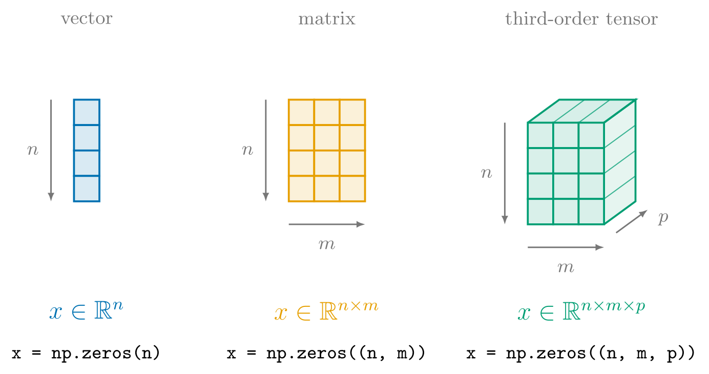
That is, they are arrays with multiple dimensionsrank,
enabling the representation of scalarsscalar, vectorsvector, matricesmatrix, and arbitrary tensorstensor of arbitrary rank.
In the case of probs, it’s a vector with support in ,
which we can verify with the two key properties of an ndarray, namely ndarray.shape and ndarray.dtype:
import numpy as np

# The same GPT-2 output distribution p(w | "Hello world, nice to") from above, top 10 of 50257 words
tokens = ["see", " meet", " hear", " have", " be", " know", " you", " talk", " say", " get"]
probs = np.array([0.3169, 0.1268, 0.1246, 0.1046, 0.0471, 0.0352, 0.0320, 0.0128, 0.0114, 0.0067])

print("gpt-2's output distribution is stored with an np.ndarray rather than a vanilla python list")
print(f"probs.shape {type(probs.shape)}: {probs.shape}")
print(f"probs.dtype {type(probs.dtype)}: {probs.dtype}")
my_tuple = (3, 4, 5)
my_tuple[0] = 2
TypeError: 'tuple' object does not support item assignment
x_reshape.shape, x_reshape.ndim, x_reshape.T
((2, 3),
 2,
 array([[5, 4],
        [2, 5],
        [3, 6]]))
np.sqrt(x)
array([2.24, 1.41, 1.73, 2. , 2.24, 2.45])
Where probs.shape.shape and probs.dtype.dtype evaluating to (10,) and dtype64 respectively means
it’s a vector with support in
whose real values are being approximately represented with double precision floating point numbers.
Another important attribute is ndarray.ndim.ndim, which is len(probs.shape) and reports the rank of an array. Since probs.ndim evaluates to 1, it has a rank of 1, or equivalently, is a vector.row major (todo)row major (todo)
col major (todo)col major (todo)
(todo, resulting tensor from .reshape() aliases the same underlying storage with different shape and strides. )
Warning
ndarray.ndimattribute.
So, an array whosendarray.ndimevaluates to 2 is not some vector but rather, an array that is some matrix , where and are unknown sincendarray.shapewas not supplied. Conversely, a multidimensional array is not simply a flat array with arbitrary length to corresponding to any vector in , but rather an array with arbitrary rank corresponding to any tensor . That is, multidimensional arrays are more accurately described as multirank arrays!
Returning to the focal point of probability and GPT-2’s conditional distribution ,
we now know that it corresponds with an ndarray whose .shape is (50256,),
or in other words some vector .
More generally, an ndarray with .shape of (V),
corresponds to a vector with a support , where is the vocabulary.
(todo: context-length is dimensionality of ).
For convenience sake, we analyzed the top 10 probabilities with an ndarray whose .shape was (10,),
which corresponded to a vector .
outcomes -> events
- todo eventevent
- todo probability of ORprobability of OR
- todo probability of ANDprobability of AND
- todo sum rulesum rule
import numpy as np

# The same GPT-2 output distribution p(w | "Hello world, nice to") from above, top 10 of 50257 words
tokens = ["see", "meet", "hear", "have", "be", "know", "you", "talk", "say", "get"]
probs = np.array([0.3169, 0.1268, 0.1246, 0.1046, 0.0471, 0.0352, 0.0320, 0.0128, 0.0114, 0.0067])

tokens_start_with_h_or_s_and_contains_a_probs = []
for token, prob in zip(tokens, probs):
    stripped = token.strip()
    starts_with_h = stripped.startswith("h")
    starts_with_s = stripped.startswith("s")
    contains_a = "a" in stripped
    if (starts_with_h or starts_with_s) and contains_a:
        tokens_start_with_h_or_s_and_contains_a_probs.append(prob)

prob_starts_with_h_or_s_and_contains_a = sum(tokens_start_with_h_or_s_and_contains_a_probs)

print(f"probability that word starts with letter h: {prob_starts_with_h}")
print(f"probability that word starts with letter s: {prob_starts_with_s}")
print(f"probability that word starts with letter h or s: {prob_starts_with_h + prob_starts_with_s}")
print(f"probability that word starts with letter h or s, and contains letter a: {prob_starts_with_h_or_s_and_contains_a}")
(todo..numpy..vectorization)
So when you ask an LLM a question, it generates a full answer (with many sentences) word by word by repeating the following loop:
- evaluating the probability of the next word conditioned on the input
- selecting (or sampling) a word. halt if the word is the special END word.
- appending it to the existing text, and evaluating the probability again with the modified input
Now that you understand the basics of language modeling, the trillion dollar question is how to produce such a conditional distribution ? In some sense that’s all there is to large language models.
1.2 Next Token Prediction is Classification
In which we introduce the terminology of software 2.0 in the context of language modeling, implement our first language model with biased histograms following the work of Andrey Markov and Claude Shannon in the early 20th century, evaluate said model with todo, and understand intelligence more broadly as compression.
1.2.1 The Estimation of Software 2.0
After §1.1 From Certain to Uncertain Knowledge,
you are now initiated with the basics of language modeling where models such as GPT-2 produce a conditional distribution
of a sentence’s next word given those that have already occured, namely .
For instance, with the input text "Hello world, nice to meet" as the history ,
GPT-2 produces the following distribution with an ndarray of .shape (V,) which represents a vector with support in .
Because we are only taking the top 10 most likely words however, .shape is (10,) with support in .
We now shift our attention to implementing language models like GPT-2 that can produce such a conditional distribution (todo).
We will incrementally increase the expressivity of our models culiminating with GPT-2’s transformer architecture in Part II. Deep Neural Networks. But for now, we start with the basics and return to first principles.
As mentioned in the previous chapter, large language models are trained using methods from the discipline of deep learningdeep learning, which in turn are based in machine learningmachine learning, which in turn are based in statistical learningstatistical learningActually, the implementation of learning is not just limited to the stochastic and infinitely continuous methods of software 2.0, more classically known as connectionism. It’s also possible to implement with logical and finitely discrete methods of software 1.0 (symbolism), albeit with much less success. i.e inductive logic programming: https://en.wikipedia.org/wiki/Inductive_logic_programming., which in turn are based in statistical inferencestatistical inference, which in turn employs the use of statistical estimationstatistical estimation. Roughly speaking, people in the business of estimation like AI researchers at frontier labs are given data (in statistical jargon, observe samples) such as the internet and would like to estimate distributions (of the population) from said data, namely a just like GPT-2. Estimation of distributions is one possible activity of making inferences from data — as opposed to simply describing data See https://en.wikipedia.org/wiki/Descriptive_statistics. — another useful form of inference is hypothesis testingSee https://en.wikipedia.org/wiki/Statistical_hypothesis_test., the process of deciding whether observed data provide sufficient evidence to reject a null hypothesis. The process of estimating distributions however serves as the heart of machine learning and deep learning, and since distributions are functions of type , estimating distributions is also commonly known as function approximationfunction approximation.
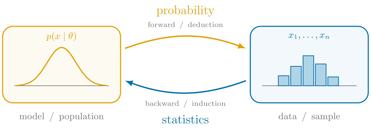
Once a distribution like is inferred from data by research labs, users can use such a distribution in order to generate sentences (which is why this most recent wave of statistical methods from software 2.0 is coloquially known as genaigenai, other previous monikers being big databig data, data miningdata mining, data sciencedata science, and pattern recognitionpattern recognition) with an inference loop, namely predicting a distribution over the next token, sampling and appending a token to the history and repeat. Generally speaking, the difference in direction of estimating a distribution from data vs generating data from a distribution is the primary distinction between probability and statistics, although the line as we will soon see gets quite blurry in the same way traditional data and function blurs with software 1.0. This distinction between the two is more broadly known as the difference between analysisanalysis and synthesissynthesisSee https://plato.stanford.edu/entries/analytic-synthetic/. Researchers analyze the observed data of the internet and recover an estimated distribution whereas users synthesize data and generate sentences. Sometimes they are referred to with direction in time: synthesis is the forward direction whereas analysis is the backward or inverse. Throughout the book, we will incrementally explore increasingly expressive languge models that can do a better job at recovering from data.
The availibility of said data determines the regime of statistical learning. That is, if sample data is available in the form of input-output pairs , then the regime is known to be supervised learningsupervised learning, for the machine that is trying to learn a distribution via induction is being supervised with the expected outputs, whereas the regime where such data is unavailable is known as unsupervised learningunsupervised learning. Whereas in unsupervised learning the goal of inference is that of understanding (todo, foreshadow ebm?) like clustering or dimensionality reduction, with supervised learning the goal is the aforementioned statistical estimation of a function that predicts the expected output, or supervision. (TODO). For instance, with the following supervised dataset:
the goal of language modelling then is to estimate some function that when given input text, predicts the next word.
- Previously we’ve denoted the conditional distribution of a language model as as the probability of the next word of a sentence given some history, where the next word is the output and the given history is the input.
Moreover, the regime of supervised learning is further refined depending on the kind of output the estimated function is predicting. In the case of a categorical output, the supervised learning is known as classificationclassification for the machine’s goal (the estimated function’s output) is trying to classify the output’s category. Language modelling in particular is considered classification because the next-token prediction performed by the estimated distribution is classifying. This stands in contrast to the case when the output the estimated function is predicting is quantitative, which is known as regressionregression.
- (recall that where the set V is the language model’s vocabulary),
- Because the type of the output is finitely discrete which stands in contrast to when the type of the output is infintely continuous such as
- If the type of the output is infintely continuous like , then the supervised learning is said to be of regressionregression, which stands in contrast to when the type of output is discretely finite like , in which supervised learning is said considered to be of
Somewhat more confusingly, depending on the domain or context of statistical modeling, the terminology for inputs and outputs might be further refined. That is, independent variableindependent variable and dependent variablesdependent variable, as well as predictorspredictors and responsesresponses in the context of ___. They can also be referred to as featuresfeatures and targetstargets. The difficulty of naming is not limited to the discipline of programmingSee https://martinfowler.com/bliki/TwoHardThings.html. Whatever you want to call them, at the heart of statical learning, machine learning and deep learning is the activity of estimation, or approximations functions with inputs and outputs. two cultures of statisticstwo cultures of statistics
Warning
1.2.2 Non-Parametric Histogram with Markov Assumption
So how do we recover the distribution Rather than strive for perfection, we can achieve the good by introducing some biasbias, known as the Markov assumptionmarkov assumption.
- sitll intractable estimate full conditionals by counting relative frequencies of truncated conditional (markov assumption)
- relative frequency is the MLE estimate
- global vs local distinction. distribution over sentences vs words
a bigram character-level language model adapted from karpathy
dataset = open('./data/names.txt', 'r').read().splitlines()
N = len(dataset)

print("--- TRAINING (counting p(w|h) with python dict ---")
# Histogram (counting frequencies) is the most precise model for training set. it *is* the training set. but it generalizes poorly.
counts_dict = {}
for di in dataset:
  di_normalized = ['<S>'] + list(di) + ['<E>']
  for h,w in zip(di_normalized, di_normalized[1:]): # in the case of bigrams h is a single character, so we can simply zip two strings to get a pair of characters
    # print(h, w)
    counts_dict[(h,w)] = counts_dict.get((h,w), 0) + 1
sorted_counts_dict = sorted(counts_dict.items(), key = lambda x: -x[1])
print("2D (w,h) histogram using python's dict:\n", sorted_counts_dict)
--- TRAINING (counting p(w|h) with python dict ---
2D (w,h) histogram using python's dict:
 [(('n', '<E>'), 6763), (('a', '<E>'), 6640), (('a', 'n'), 5438), (('<S>', 'a'), 4410), (('e', '<E>'), 3983), (('a', 'r'), 3264), (('e', 'l'), 3248), (('r', 'i'), 3033), (('n', 'a'), 2977), (('<S>', 'k'), 2963), (('l', 'e'), 2921), (('e', 'n'), 2675), (('l', 'a'), 2623), (('m', 'a'), 2590), (('<S>', 'm'), 2538), (('a', 'l'), 2528), (('i', '<E>'), 2489), (('l', 'i'), 2480), (('i', 'a'), 2445), (('<S>', 'j'), 2422), (('o', 'n'), 2411), (('h', '<E>'), 2409), (('r', 'a'), 2356), (('a', 'h'), 2332), (('h', 'a'), 2244), (('y', 'a'), 2143), (('i', 'n'), 2126), (('<S>', 's'), 2055), (('a', 'y'), 2050), (('y', '<E>'), 2007), (('e', 'r'), 1958), (('n', 'n'), 1906), (('y', 'n'), 1826), (('k', 'a'), 1731), (('n', 'i'), 1725), (('r', 'e'), 1697), (('<S>', 'd'), 1690), (('i', 'e'), 1653), (('a', 'i'), 1650), (('<S>', 'r'), 1639), (('a', 'm'), 1634), (('l', 'y'), 1588), (('<S>', 'l'), 1572), (('<S>', 'c'), 1542), (('<S>', 'e'), 1531), (('j', 'a'), 1473), (('r', '<E>'), 1377), (('n', 'e'), 1359), (('l', 'l'), 1345), (('i', 'l'), 1345), (('i', 's'), 1316), (('l', '<E>'), 1314), (('<S>', 't'), 1308), (('<S>', 'b'), 1306), (('d', 'a'), 1303), (('s', 'h'), 1285), (('d', 'e'), 1283), (('e', 'e'), 1271), (('m', 'i'), 1256), (('s', 'a'), 1201), (('s', '<E>'), 1169), (('<S>', 'n'), 1146), (('a', 's'), 1118), (('y', 'l'), 1104), (('e', 'y'), 1070), (('o', 'r'), 1059), (('a', 'd'), 1042), (('t', 'a'), 1027), (('<S>', 'z'), 929), (('v', 'i'), 911), (('k', 'e'), 895), (('s', 'e'), 884), (('<S>', 'h'), 874), (('r', 'o'), 869), (('e', 's'), 861), (('z', 'a'), 860), (('o', '<E>'), 855), (('i', 'r'), 849), (('b', 'r'), 842), (('a', 'v'), 834), (('m', 'e'), 818), (('e', 'i'), 818), (('c', 'a'), 815), (('i', 'y'), 779), (('r', 'y'), 773), (('e', 'm'), 769), (('s', 't'), 765), (('h', 'i'), 729), (('t', 'e'), 716), (('n', 'd'), 704), (('l', 'o'), 692), (('a', 'e'), 692), (('a', 't'), 687), (('s', 'i'), 684), (('e', 'a'), 679), (('d', 'i'), 674), (('h', 'e'), 674), (('<S>', 'g'), 669), (('t', 'o'), 667), (('c', 'h'), 664), (('b', 'e'), 655), (('t', 'h'), 647), (('v', 'a'), 642), (('o', 'l'), 619), (('<S>', 'i'), 591), (('i', 'o'), 588), (('e', 't'), 580), (('v', 'e'), 568), (('a', 'k'), 568), (('a', 'a'), 556), (('c', 'e'), 551), (('a', 'b'), 541), (('i', 't'), 541), (('<S>', 'y'), 535), (('t', 'i'), 532), (('s', 'o'), 531), (('m', '<E>'), 516), (('d', '<E>'), 516), (('<S>', 'p'), 515), (('i', 'c'), 509), (('k', 'i'), 509), (('o', 's'), 504), (('n', 'o'), 496), (('t', '<E>'), 483), (('j', 'o'), 479), (('u', 's'), 474), (('a', 'c'), 470), (('n', 'y'), 465), (('e', 'v'), 463), (('s', 's'), 461), (('m', 'o'), 452), (('i', 'k'), 445), (('n', 't'), 443), (('i', 'd'), 440), (('j', 'e'), 440), (('a', 'z'), 435), (('i', 'g'), 428), (('i', 'm'), 427), (('r', 'r'), 425), (('d', 'r'), 424), (('<S>', 'f'), 417), (('u', 'r'), 414), (('r', 'l'), 413), (('y', 's'), 401), (('<S>', 'o'), 394), (('e', 'd'), 384), (('a', 'u'), 381), (('c', 'o'), 380), (('k', 'y'), 379), (('d', 'o'), 378), (('<S>', 'v'), 376), (('t', 't'), 374), (('z', 'e'), 373), (('z', 'i'), 364), (('k', '<E>'), 363), (('g', 'h'), 360), (('t', 'r'), 352), (('k', 'o'), 344), (('t', 'y'), 341), (('g', 'e'), 334), (('g', 'a'), 330), (('l', 'u'), 324), (('b', 'a'), 321), (('d', 'y'), 317), (('c', 'k'), 316), (('<S>', 'w'), 307), (('k', 'h'), 307), (('u', 'l'), 301), (('y', 'e'), 301), (('y', 'r'), 291), (('m', 'y'), 287), (('h', 'o'), 287), (('w', 'a'), 280), (('s', 'l'), 279), (('n', 's'), 278), (('i', 'z'), 277), (('u', 'n'), 275), (('o', 'u'), 275), (('n', 'g'), 273), (('y', 'd'), 272), (('c', 'i'), 271), (('y', 'o'), 271), (('i', 'v'), 269), (('e', 'o'), 269), (('o', 'm'), 261), (('r', 'u'), 252), (('f', 'a'), 242), (('b', 'i'), 217), (('s', 'y'), 215), (('n', 'c'), 213), (('h', 'y'), 213), (('p', 'a'), 209), (('r', 't'), 208), (('q', 'u'), 206), (('p', 'h'), 204), (('h', 'r'), 204), (('j', 'u'), 202), (('g', 'r'), 201), (('p', 'e'), 197), (('n', 'l'), 195), (('y', 'i'), 192), (('g', 'i'), 190), (('o', 'd'), 190), (('r', 's'), 190), (('r', 'd'), 187), (('h', 'l'), 185), (('s', 'u'), 185), (('a', 'x'), 182), (('e', 'z'), 181), (('e', 'k'), 178), (('o', 'v'), 176), (('a', 'j'), 175), (('o', 'h'), 171), (('u', 'e'), 169), (('m', 'm'), 168), (('a', 'g'), 168), (('h', 'u'), 166), (('x', '<E>'), 164), (('u', 'a'), 163), (('r', 'm'), 162), (('a', 'w'), 161), (('f', 'i'), 160), (('z', '<E>'), 160), (('u', '<E>'), 155), (('u', 'm'), 154), (('e', 'c'), 153), (('v', 'o'), 153), (('e', 'h'), 152), (('p', 'r'), 151), (('d', 'd'), 149), (('o', 'a'), 149), (('w', 'e'), 149), (('w', 'i'), 148), (('y', 'm'), 148), (('z', 'y'), 147), (('n', 'z'), 145), (('y', 'u'), 141), (('r', 'n'), 140), (('o', 'b'), 140), (('k', 'l'), 139), (('m', 'u'), 139), (('l', 'd'), 138), (('h', 'n'), 138), (('u', 'd'), 136), (('<S>', 'x'), 134), (('t', 'l'), 134), (('a', 'f'), 134), (('o', 'e'), 132), (('e', 'x'), 132), (('e', 'g'), 125), (('f', 'e'), 123), (('z', 'l'), 123), (('u', 'i'), 121), (('v', 'y'), 121), (('e', 'b'), 121), (('r', 'h'), 121), (('j', 'i'), 119), (('o', 't'), 118), (('d', 'h'), 118), (('h', 'm'), 117), (('c', 'l'), 116), (('o', 'o'), 115), (('y', 'c'), 115), (('o', 'w'), 114), (('o', 'c'), 114), (('f', 'r'), 114), (('b', '<E>'), 114), (('m', 'b'), 112), (('z', 'o'), 110), (('i', 'b'), 110), (('i', 'u'), 109), (('k', 'r'), 109), (('g', '<E>'), 108), (('y', 'v'), 106), (('t', 'z'), 105), (('b', 'o'), 105), (('c', 'y'), 104), (('y', 't'), 104), (('u', 'b'), 103), (('u', 'c'), 103), (('x', 'a'), 103), (('b', 'l'), 103), (('o', 'y'), 103), (('x', 'i'), 102), (('i', 'f'), 101), (('r', 'c'), 99), (('c', '<E>'), 97), (('m', 'r'), 97), (('n', 'u'), 96), (('o', 'p'), 95), (('i', 'h'), 95), (('k', 's'), 95), (('l', 's'), 94), (('u', 'k'), 93), (('<S>', 'q'), 92), (('d', 'u'), 92), (('s', 'm'), 90), (('r', 'k'), 90), (('i', 'x'), 89), (('v', '<E>'), 88), (('y', 'k'), 86), (('u', 'w'), 86), (('g', 'u'), 85), (('b', 'y'), 83), (('e', 'p'), 83), (('g', 'o'), 83), (('s', 'k'), 82), (('u', 't'), 82), (('a', 'p'), 82), (('e', 'f'), 82), (('i', 'i'), 82), (('r', 'v'), 80), (('f', '<E>'), 80), (('t', 'u'), 78), (('y', 'z'), 78), (('<S>', 'u'), 78), (('l', 't'), 77), (('r', 'g'), 76), (('c', 'r'), 76), (('i', 'j'), 76), (('w', 'y'), 73), (('z', 'u'), 73), (('l', 'v'), 72), (('h', 't'), 71), (('j', '<E>'), 71), (('x', 't'), 70), (('o', 'i'), 69), (('e', 'u'), 69), (('o', 'k'), 68), (('b', 'd'), 65), (('a', 'o'), 63), (('p', 'i'), 61), (('s', 'c'), 60), (('d', 'l'), 60), (('l', 'm'), 60), (('a', 'q'), 60), (('f', 'o'), 60), (('p', 'o'), 59), (('n', 'k'), 58), (('w', 'n'), 58), (('u', 'h'), 58), (('e', 'j'), 55), (('n', 'v'), 55), (('s', 'r'), 55), (('o', 'z'), 54), (('i', 'p'), 53), (('l', 'b'), 52), (('i', 'q'), 52), (('w', '<E>'), 51), (('m', 'c'), 51), (('s', 'p'), 51), (('e', 'w'), 50), (('k', 'u'), 50), (('v', 'r'), 48), (('u', 'g'), 47), (('o', 'x'), 45), (('u', 'z'), 45), (('z', 'z'), 45), (('j', 'h'), 45), (('b', 'u'), 45), (('o', 'g'), 44), (('n', 'r'), 44), (('f', 'f'), 44), (('n', 'j'), 44), (('z', 'h'), 43), (('c', 'c'), 42), (('r', 'b'), 41), (('x', 'o'), 41), (('b', 'h'), 41), (('p', 'p'), 39), (('x', 'l'), 39), (('h', 'v'), 39), (('b', 'b'), 38), (('m', 'p'), 38), (('x', 'x'), 38), (('u', 'v'), 37), (('x', 'e'), 36), (('w', 'o'), 36), (('c', 't'), 35), (('z', 'm'), 35), (('t', 's'), 35), (('m', 's'), 35), (('c', 'u'), 35), (('o', 'f'), 34), (('u', 'x'), 34), (('k', 'w'), 34), (('p', '<E>'), 33), (('g', 'l'), 32), (('z', 'r'), 32), (('d', 'n'), 31), (('g', 't'), 31), (('g', 'y'), 31), (('h', 's'), 31), (('x', 's'), 31), (('g', 's'), 30), (('x', 'y'), 30), (('y', 'g'), 30), (('d', 'm'), 30), (('d', 's'), 29), (('h', 'k'), 29), (('y', 'x'), 28), (('q', '<E>'), 28), (('g', 'n'), 27), (('y', 'b'), 27), (('g', 'w'), 26), (('n', 'h'), 26), (('k', 'n'), 26), (('g', 'g'), 25), (('d', 'g'), 25), (('l', 'c'), 25), (('r', 'j'), 25), (('w', 'u'), 25), (('l', 'k'), 24), (('m', 'd'), 24), (('s', 'w'), 24), (('s', 'n'), 24), (('h', 'd'), 24), (('w', 'h'), 23), (('y', 'j'), 23), (('y', 'y'), 23), (('r', 'z'), 23), (('d', 'w'), 23), (('w', 'r'), 22), (('t', 'n'), 22), (('l', 'f'), 22), (('y', 'h'), 22), (('r', 'w'), 21), (('s', 'b'), 21), (('m', 'n'), 20), (('f', 'l'), 20), (('w', 's'), 20), (('k', 'k'), 20), (('h', 'z'), 20), (('g', 'd'), 19), (('l', 'h'), 19), (('n', 'm'), 19), (('x', 'z'), 19), (('u', 'f'), 19), (('f', 't'), 18), (('l', 'r'), 18), (('p', 't'), 17), (('t', 'c'), 17), (('k', 't'), 17), (('d', 'v'), 17), (('u', 'p'), 16), (('p', 'l'), 16), (('l', 'w'), 16), (('p', 's'), 16), (('o', 'j'), 16), (('r', 'q'), 16), (('y', 'p'), 15), (('l', 'p'), 15), (('t', 'v'), 15), (('r', 'p'), 14), (('l', 'n'), 14), (('e', 'q'), 14), (('f', 'y'), 14), (('s', 'v'), 14), (('u', 'j'), 14), (('v', 'l'), 14), (('q', 'a'), 13), (('u', 'y'), 13), (('q', 'i'), 13), (('w', 'l'), 13), (('p', 'y'), 12), (('y', 'f'), 12), (('c', 'q'), 11), (('j', 'r'), 11), (('n', 'w'), 11), (('n', 'f'), 11), (('t', 'w'), 11), (('m', 'z'), 11), (('u', 'o'), 10), (('f', 'u'), 10), (('l', 'z'), 10), (('h', 'w'), 10), (('u', 'q'), 10), (('j', 'y'), 10), (('s', 'z'), 10), (('s', 'd'), 9), (('j', 'l'), 9), (('d', 'j'), 9), (('k', 'm'), 9), (('r', 'f'), 9), (('h', 'j'), 9), (('v', 'n'), 8), (('n', 'b'), 8), (('i', 'w'), 8), (('h', 'b'), 8), (('b', 's'), 8), (('w', 't'), 8), (('w', 'd'), 8), (('v', 'v'), 7), (('v', 'u'), 7), (('j', 's'), 7), (('m', 'j'), 7), (('f', 's'), 6), (('l', 'g'), 6), (('l', 'j'), 6), (('j', 'w'), 6), (('n', 'x'), 6), (('y', 'q'), 6), (('w', 'k'), 6), (('g', 'm'), 6), (('x', 'u'), 5), (('m', 'h'), 5), (('m', 'l'), 5), (('j', 'm'), 5), (('c', 's'), 5), (('j', 'v'), 5), (('n', 'p'), 5), (('d', 'f'), 5), (('x', 'd'), 5), (('z', 'b'), 4), (('f', 'n'), 4), (('x', 'c'), 4), (('m', 't'), 4), (('t', 'm'), 4), (('z', 'n'), 4), (('z', 't'), 4), (('p', 'u'), 4), (('c', 'z'), 4), (('b', 'n'), 4), (('z', 's'), 4), (('f', 'w'), 4), (('d', 't'), 4), (('j', 'd'), 4), (('j', 'c'), 4), (('y', 'w'), 4), (('v', 'k'), 3), (('x', 'w'), 3), (('t', 'j'), 3), (('c', 'j'), 3), (('q', 'w'), 3), (('g', 'b'), 3), (('o', 'q'), 3), (('r', 'x'), 3), (('d', 'c'), 3), (('g', 'j'), 3), (('x', 'f'), 3), (('z', 'w'), 3), (('d', 'k'), 3), (('u', 'u'), 3), (('m', 'v'), 3), (('c', 'x'), 3), (('l', 'q'), 3), (('p', 'b'), 2), (('t', 'g'), 2), (('q', 's'), 2), (('t', 'x'), 2), (('f', 'k'), 2), (('b', 't'), 2), (('j', 'n'), 2), (('k', 'c'), 2), (('z', 'k'), 2), (('s', 'j'), 2), (('s', 'f'), 2), (('z', 'j'), 2), (('n', 'q'), 2), (('f', 'z'), 2), (('h', 'g'), 2), (('w', 'w'), 2), (('k', 'j'), 2), (('j', 'k'), 2), (('w', 'm'), 2), (('z', 'c'), 2), (('z', 'v'), 2), (('w', 'f'), 2), (('q', 'm'), 2), (('k', 'z'), 2), (('j', 'j'), 2), (('z', 'p'), 2), (('j', 't'), 2), (('k', 'b'), 2), (('m', 'w'), 2), (('h', 'f'), 2), (('c', 'g'), 2), (('t', 'f'), 2), (('h', 'c'), 2), (('q', 'o'), 2), (('k', 'd'), 2), (('k', 'v'), 2), (('s', 'g'), 2), (('z', 'd'), 2), (('q', 'r'), 1), (('d', 'z'), 1), (('p', 'j'), 1), (('q', 'l'), 1), (('p', 'f'), 1), (('q', 'e'), 1), (('b', 'c'), 1), (('c', 'd'), 1), (('m', 'f'), 1), (('p', 'n'), 1), (('w', 'b'), 1), (('p', 'c'), 1), (('h', 'p'), 1), (('f', 'h'), 1), (('b', 'j'), 1), (('f', 'g'), 1), (('z', 'g'), 1), (('c', 'p'), 1), (('p', 'k'), 1), (('p', 'm'), 1), (('x', 'n'), 1), (('s', 'q'), 1), (('k', 'f'), 1), (('m', 'k'), 1), (('x', 'h'), 1), (('g', 'f'), 1), (('v', 'b'), 1), (('j', 'p'), 1), (('g', 'z'), 1), (('v', 'd'), 1), (('d', 'b'), 1), (('v', 'h'), 1), (('h', 'h'), 1), (('g', 'v'), 1), (('d', 'q'), 1), (('x', 'b'), 1), (('w', 'z'), 1), (('h', 'q'), 1), (('j', 'b'), 1), (('x', 'm'), 1), (('w', 'g'), 1), (('t', 'b'), 1), (('z', 'x'), 1)]
print("--- TRAINING (counting p(w|h) with numpy ndarray (NxN) ---")
# We will now construct the same 2d histogram, but with numpy's ndarray instead of python's dict
# Because numpy's ndarray uses numerical indices to index into, we need to create a dict[str,int]
# so that when we loop over (w,h) pairs within a word we can update the count at the correct location
import numpy as np
vocab = sorted(list(set(''.join(dataset)))) # construct vocab
c2i = {c:i+1 for i,c in enumerate(vocab)}                      # construct map<char,ord>
c2i['.'] = 0                                                                            # with . as the start token and end token, to remove counting freq of (<E>*) and (*<S>) which are all 0
V = len(c2i)                                                                   # evaluate the vocab len V
C_VV = np.zeros((V,V), dtype=np.int32)      # and use V to construct C_VV

# Now we can proceed
for di in dataset:
  di_normalized = ['.'] + list(di) + ['.']
  for h,w in zip(di_normalized, di_normalized[1:]):
    print(h,w)
    h_index, w_index = c2i[h], c2i[w]                                         # use map<char, ord> to lookup the coordinate index needed for C_VV
    C_VV[h_index, w_index] += 1                                                         # update C_VV
print("2D (xt,xt-1) histogram using numpy dict:\n", C_VV)

# normalize counts C_VV to probs P_VV
C_VVf32 = (C_VV+1).astype(np.float32)           # inductive bias (locally smooth)
s_V1 = C_VVf32.sum(axis=1,keepdims=True)              # reduce along axis=1 because we want p(y|x) not p(x|y)
P_VV = C_VVf32 / s_V1                                                                   # (V, V) / (V, 1) broadcasts

# for P_VV, the elements are the counts of bigrams (h,w) accessed by indexing with ord(h) at axis=0 and ord(w) at axis=1
# now, since numpy's ndarray's are row major order, axis=0 gets printed vertically from up to down while axis=1 gets printed horizontally from left to right
i2c = {i:c for c,i in c2i.items()}  # invert map<char, ord> to map<ord, char> because looping with enumerate provides access to indices
header = '    ' + ' '.join(f'{i2c[y_index]:>4}' for y_index in range(V))
print("2D (ord, ord) histogram using numpy ndarray")
print(header)
for w_index, row in enumerate(C_VV+1):
  h = f'{i2c[w_index]:>4}'
  print(h, ' '.join(f'{count:>4}' for count in row))
--- TRAINING (counting p(w|h) with numpy ndarray (NxN) ---
. e
e m
m m
m a
a .
. o
o l
l i
i v
v i
i a
a .
. a
a v
v a
a .
. i
i s
s a
a b
b e
e l
l l
l a
a .
. s
s o
o p
p h
h i
i a
a .
. c
c h
h a
a r
r l
l o
o t
t t
t e
e .
. m
m i
i a
a .
. a
a m
m e
e l
l i
i a
a .
. h
h a
a r
r p
p e
e r
r .
. e
e v
v e
e l
l y
y n
n .
. a
a b
b i
i g
g a
a i
i l
l .
. e
e m
m i
i l
l y
y .
. e
e l
l i
i z
z a
a b
b e
e t
t h
h .
. m
m i
i l
l a
a .
. e
e l
l l
l a
a .
. a
a v
v e
e r
r y
y .
. s
s o
o f
f i
i a
a .
. c
c a
a m
m i
i l
l a
a .
. a
a r
r i
i a
a .
. s
s c
c a
a r
r l
l e
e t
t t
t .
. v
v i
i c
c t
t o
o r
r i
i a
a .
. m
m a
a d
d i
i s
s o
o n
n .
. l
l u
u n
n a
a .
. g
g r
r a
a c
c e
e .
. c
c h
h l
l o
o e
e .
. p
p e
e n
n e
e l
l o
o p
p e
e .
. l
l a
a y
y l
l a
a .
. r
r i
i l
l e
e y
y .
. z
z o
o e
e y
y .
. n
n o
o r
r a
a .
. l
l i
i l
l y
y .
. e
e l
l e
e a
a n
n o
o r
r .
. h
h a
a n
n n
n a
a h
h .
. l
l i
i l
l l
l i
i a
a n
n .
. a
a d
d d
d i
i s
s o
o n
n .
. a
a u
u b
b r
r e
e y
y .
. e
e l
l l
l i
i e
e .
. s
s t
t e
e l
l l
l a
a .
. n
n a
a t
t a
a l
l i
i e
e .
. z
z o
o e
e .
. l
l e
e a
a h
h .
. h
h a
a z
z e
e l
l .
. v
v i
i o
o l
l e
e t
t .
. a
a u
u r
r o
o r
r a
a .
. s
s a
a v
v a
a n
n n
n a
a h
h .
. a
a u
u d
d r
r e
e y
y .
. b
b r
r o
o o
o k
k l
l y
y n
n .
. b
b e
e l
l l
l a
a .
. c
c l
l a
a i
i r
r e
e .
. s
s k
k y
y l
l a
a r
r .
. l
l u
u c
c y
y .
. p
p a
a i
i s
s l
l e
e y
y .
. e
e v
v e
e r
r l
l y
y .
. a
a n
n n
n a
a .
. c
c a
a r
r o
o l
l i
i n
n e
e .
. n
n o
o v
v a
a .
. g
g e
e n
n e
e s
s i
i s
s .
. e
e m
m i
i l
l i
i a
a .
. k
k e
e n
n n
n e
e d
d y
y .
. s
s a
a m
m a
a n
n t
t h
h a
a .
. m
m a
a y
y a
a .
. w
w i
i l
l l
l o
o w
w .
. k
k i
i n
n s
s l
l e
e y
y .
. n
n a
a o
o m
m i
i .
. a
a a
a l
l i
i y
y a
a h
h .
. e
e l
l e
e n
n a
a .
. s
s a
a r
r a
a h
h .
. a
a r
r i
i a
a n
n a
a .
. a
a l
l l
l i
i s
s o
o n
n .
. g
g a
a b
b r
r i
i e
e l
l l
l a
a .
. a
a l
l i
i c
c e
e .
. m
m a
a d
d e
e l
l y
y n
n .
. c
c o
o r
r a
a .
. r
r u
u b
b y
y .
. e
e v
v a
a .
. s
s e
e r
r e
e n
n i
i t
t y
y .
. a
a u
u t
t u
u m
m n
n .
. a
a d
d e
e l
l i
i n
n e
e .
. h
h a
a i
i l
l e
e y
y .
. g
g i
i a
a n
n n
n a
a .
. v
v a
a l
l e
e n
n t
t i
i n
n a
a .
. i
i s
s l
l a
a .
. e
e l
l i
i a
a n
n a
a .
. q
q u
u i
i n
n n
n .
. n
n e
e v
v a
a e
e h
h .
. i
i v
v y
y .
. s
s a
a d
d i
i e
e .
. p
p i
i p
p e
e r
r .
. l
l y
y d
d i
i a
a .
. a
a l
l e
e x
x a
a .
. j
j o
o s
s e
e p
p h
h i
i n
n e
e .
. e
e m
m e
e r
r y
y .
. j
j u
u l
l i
i a
a .
. d
d e
e l
l i
i l
l a
a h
h .
. a
a r
r i
i a
a n
n n
n a
a .
. v
v i
i v
v i
i a
a n
n .
. k
k a
a y
y l
l e
e e
e .
. s
s o
o p
p h
h i
i e
e .
. b
b r
r i
i e
e l
l l
l e
e .
. m
m a
a d
d e
e l
l i
i n
n e
e .
. p
p e
e y
y t
t o
o n
n .
. r
r y
y l
l e
e e
e .
. c
c l
l a
a r
r a
a .
. h
h a
a d
d l
l e
e y
y .
. m
m e
e l
l a
a n
n i
i e
e .
. m
m a
a c
c k
k e
e n
n z
z i
i e
e .
. r
r e
e a
a g
g a
a n
n .
. a
a d
d a
a l
l y
y n
n n
n .
. l
l i
i l
l i
i a
a n
n a
a .
. a
a u
u b
b r
r e
e e
e .
. j
j a
a d
d e
e .
. k
k a
a t
t h
h e
e r
r i
i n
n e
e .
. i
i s
s a
a b
b e
e l
l l
l e
e .
. n
n a
a t
t a
a l
l i
i a
a .
. r
r a
a e
e l
l y
y n
n n
n .
. m
m a
a r
r i
i a
a .
. a
a t
t h
h e
e n
n a
a .
. x
x i
i m
m e
e n
n a
a .
. a
a r
r y
y a
a .
. l
l e
e i
i l
l a
a n
n i
i .
. t
t a
a y
y l
l o
o r
r .
. f
f a
a i
i t
t h
h .
. r
r o
o s
s e
e .
. k
k y
y l
l i
i e
e .
. a
a l
l e
e x
x a
a n
n d
d r
r a
a .
. m
m a
a r
r y
y .
. m
m a
a r
r g
g a
a r
r e
e t
t .
. l
l y
y l
l a
a .
. a
a s
s h
h l
l e
e y
y .
. a
a m
m a
a y
y a
a .
. e
e l
l i
i z
z a
a .
. b
b r
r i
i a
a n
n n
n a
a .
. b
b a
a i
i l
l e
e y
y .
. a
a n
n d
d r
r e
e a
a .
. k
k h
h l
l o
o e
e .
. j
j a
a s
s m
m i
i n
n e
e .
. m
m e
e l
l o
o d
d y
y .
. i
i r
r i
i s
s .
. i
i s
s a
a b
b e
e l
l .
. n
n o
o r
r a
a h
h .
. a
a n
n n
n a
a b
b e
e l
l l
l e
e .
. v
v a
a l
l e
e r
r i
i a
a .
. e
e m
m e
e r
r s
s o
o n
n .
. a
a d
d a
a l
l y
y n
n .
. r
r y
y l
l e
e i
i g
g h
h .
. e
e d
d e
e n
n .
. e
e m
m e
e r
r s
s y
y n
n .
. a
a n
n a
a s
s t
t a
a s
s i
i a
a .
. k
k a
a y
y l
l a
a .
. a
a l
l y
y s
s s
s a
a .
. j
j u
u l
l i
i a
a n
n a
a .
. c
c h
h a
a r
r l
l i
i e
e .
. e
e s
s t
t h
h e
e r
r .
. a
a r
r i
i e
e l
l .
. c
c e
e c
c i
i l
l i
i a
a .
. v
v a
a l
l e
e r
r i
i e
e .
. a
a l
l i
i n
n a
a .
. m
m o
o l
l l
l y
y .
. r
r e
e e
e s
s e
e .
. a
a l
l i
i y
y a
a h
h .
. l
l i
i l
l l
l y
y .
. p
p a
a r
r k
k e
e r
r .
. f
f i
i n
n l
l e
e y
y .
. m
m o
o r
r g
g a
a n
n .
. s
s y
y d
d n
n e
e y
y .
. j
j o
o r
r d
d y
y n
n .
. e
e l
l o
o i
i s
s e
e .
. t
t r
r i
i n
n i
i t
t y
y .
. d
d a
a i
i s
s y
y .
. k
k i
i m
m b
b e
e r
r l
l y
y .
. l
l a
a u
u r
r e
e n
n .
. g
g e
e n
n e
e v
v i
i e
e v
v e
e .
. s
s a
a r
r a
a .
. a
a r
r a
a b
b e
e l
l l
l a
a .
. h
h a
a r
r m
m o
o n
n y
y .
. e
e l
l i
i s
s e
e .
. r
r e
e m
m i
i .
. t
t e
e a
a g
g a
a n
n .
. a
a l
l e
e x
x i
i s
s .
. l
l o
o n
n d
d o
o n
n .
. s
s l
l o
o a
a n
n e
e .
. l
l a
a i
i l
l a
a .
. l
l u
u c
c i
i a
a .
. d
d i
i a
a n
n a
a .
. j
j u
u l
l i
i e
e t
t t
t e
e .
. s
s i
i e
e n
n n
n a
a .
. e
e l
l l
l i
i a
a n
n a
a .
. l
l o
o n
n d
d y
y n
n .
. a
a y
y l
l a
a .
. c
c a
a l
l l
l i
i e
e .
. g
g r
r a
a c
c i
i e
e .
. j
j o
o s
s i
i e
e .
. a
a m
m a
a r
r a
a .
. j
j o
o c
c e
e l
l y
y n
n .
. d
d a
a n
n i
i e
e l
l a
a .
. e
e v
v e
e r
r l
l e
e i
i g
g h
h .
. m
m y
y a
a .
. r
r a
a c
c h
h e
e l
l .
. s
s u
u m
m m
m e
e r
r .
. a
a l
l a
a n
n a
a .
. b
b r
r o
o o
o k
k e
e .
. a
a l
l a
a i
i n
n a
a .
. m
m c
c k
k e
e n
n z
z i
i e
e .
. c
c a
a t
t h
h e
e r
r i
i n
n e
e .
. a
a m
m y
y .
. p
p r
r e
e s
s l
l e
e y
y .
. j
j o
o u
u r
r n
n e
e e
e .
. r
r o
o s
s a
a l
l i
i e
e .
. e
e m
m b
b e
e r
r .
. b
b r
r y
y n
n l
l e
e e
e .
. r
r o
o w
w a
a n
n .
. j
j o
o a
a n
n n
n a
a .
. p
p a
a i
i g
g e
e .
. r
r e
e b
b e
e c
c c
c a
a .
. a
a n
n a
a .
. s
s a
a w
w y
y e
e r
r .
. m
m a
a r
r i
i a
a h
h .
. n
n i
i c
c o
o l
l e
e .
. b
b r
r o
o o
o k
k l
l y
y n
n n
n .
. p
p a
a y
y t
t o
o n
n .
. m
m a
a r
r l
l e
e y
y .
. f
f i
i o
o n
n a
a .
. g
g e
e o
o r
r g
g i
i a
a .
. l
l i
i l
l a
a .
. h
h a
a r
r l
l e
e y
y .
. a
a d
d e
e l
l y
y n
n .
. a
a l
l i
i v
v i
i a
a .
. n
n o
o e
e l
l l
l e
e .
. g
g e
e m
m m
m a
a .
. v
v a
a n
n e
e s
s s
s a
a .
. j
j o
o u
u r
r n
n e
e y
y .
. m
m a
a k
k a
a y
y l
l a
a .
. a
a n
n g
g e
e l
l i
i n
n a
a .
. a
a d
d a
a l
l i
i n
n e
e .
. c
c a
a t
t a
a l
l i
i n
n a
a .
. a
a l
l a
a y
y n
n a
a .
. j
j u
u l
l i
i a
a n
n n
n a
a .
. l
l e
e i
i l
l a
a .
. l
l o
o l
l a
a .
. a
a d
d r
r i
i a
a n
n a
a .
. j
j u
u n
n e
e .
. j
j u
u l
l i
i e
e t
t .
. j
j a
a y
y l
l a
a .
. r
r i
i v
v e
e r
r .
. t
t e
e s
s s
s a
a .
. l
l i
i a
a .
. d
d a
a k
k o
o t
t a
a .
. d
d e
e l
l a
a n
n e
e y
y .
. s
s e
e l
l e
e n
n a
a .
. b
b l
l a
a k
k e
e l
l y
y .
. a
a d
d a
a .
. c
c a
a m
m i
i l
l l
l e
e .
. z
z a
a r
r a
a .
. m
m a
a l
l i
i a
a .
. h
h o
o p
p e
e .
. s
s a
a m
m a
a r
r a
a .
. v
v e
e r
r a
a .
. m
m c
c k
k e
e n
n n
n a
a .
. b
b r
r i
i e
e l
l l
l a
a .
. i
i z
z a
a b
b e
e l
l l
l a
a .
. h
h a
a y
y d
d e
e n
n .
. r
r a
a e
e g
g a
a n
n .
. m
m i
i c
c h
h e
e l
l l
l e
e .
. a
a n
n g
g e
e l
l a
a .
. r
r u
u t
t h
h .
. f
f r
r e
e y
y a
a .
. k
k a
a m
m i
i l
l a
a .
. v
v i
i v
v i
i e
e n
n n
n e
e .
. a
a s
s p
p e
e n
n .
. o
o l
l i
i v
v e
e .
. k
k e
e n
n d
d a
a l
l l
l .
. e
e l
l a
a i
i n
n a
a .
. t
t h
h e
e a
a .
. k
k a
a l
l i
i .
. d
d e
e s
s t
t i
i n
n y
y .
. a
a m
m i
i y
y a
a h
h .
. e
e v
v a
a n
n g
g e
e l
l i
i n
n e
e .
. c
c a
a l
l i
i .
. b
b l
l a
a k
k e
e .
. e
e l
l s
s i
i e
e .
. j
j u
u n
n i
i p
p e
e r
r .
. a
a l
l e
e x
x a
a n
n d
d r
r i
i a
a .
. m
m y
y l
l a
a .
. a
a r
r i
i e
e l
l l
l a
a .
. k
k a
a t
t e
e .
. m
m a
a r
r i
i a
a n
n a
a .
. l
l i
i l
l a
a h
h .
. c
c h
h a
a r
r l
l e
e e
e .
. d
d a
a l
l e
e y
y z
z a
a .
. n
n y
y l
l a
a .
. j
j a
a n
n e
e .
. m
m a
a g
g g
g i
i e
e .
. z
z u
u r
r i
i .
. a
a n
n i
i y
y a
a h
h .
. l
l u
u c
c i
i l
l l
l e
e .
. l
l e
e i
i a
a .
. m
m e
e l
l i
i s
s s
s a
a .
. a
a d
d e
e l
l a
a i
i d
d e
e .
. a
a m
m i
i n
n a
a .
. g
g i
i s
s e
e l
l l
l e
e .
. l
l e
e n
n a
a .
. c
c a
a m
m i
i l
l l
l a
a .
. m
m i
i r
r i
i a
a m
m .
. m
m i
i l
l l
l i
i e
e .
. b
b r
r y
y n
n n
n .
. g
g a
a b
b r
r i
i e
e l
l l
l e
e .
. s
s a
a g
g e
e .
. a
a n
n n
n i
i e
e .
. l
l o
o g
g a
a n
n .
. l
l i
i l
l l
l i
i a
a n
n a
a .
. h
h a
a v
v e
e n
n .
. j
j e
e s
s s
s i
i c
c a
a .
. k
k a
a i
i a
a .
. m
m a
a g
g n
n o
o l
l i
i a
a .
. a
a m
m i
i r
r a
a .
. a
a d
d e
e l
l y
y n
n n
n .
. m
m a
a k
k e
e n
n z
z i
i e
e .
. s
s t
t e
e p
p h
h a
a n
n i
i e
e .
. n
n i
i n
n a
a .
. p
p h
h o
o e
e b
b e
e .
. a
a r
r i
i e
e l
l l
l e
e .
. e
e v
v i
i e
e .
. l
l y
y r
r i
i c
c .
. a
a l
l e
e s
s s
s a
a n
n d
d r
r a
a .
. g
g a
a b
b r
r i
i e
e l
l a
a .
. p
p a
a i
i s
s l
l e
e e
e .
. r
r a
a e
e l
l y
y n
n .
. m
m a
a d
d i
i l
l y
y n
n .
. p
p a
a r
r i
i s
s .
. m
m a
a k
k e
e n
n n
n a
a .
. k
k i
i n
n l
l e
e y
y .
. g
g r
r a
a c
c e
e l
l y
y n
n .
. t
t a
a l
l i
i a
a .
. m
m a
a e
e v
v e
e .
. r
r y
y l
l i
i e
e .
. k
k i
i a
a r
r a
a .
. e
e v
v e
e l
l y
y n
n n
n .
. b
b r
r i
i n
n l
l e
e y
y .
. j
j a
a c
c q
q u
u e
e l
l i
i n
n e
e .
. l
l a
a u
u r
r a
a .
. g
g r
r a
a c
c e
e l
l y
y n
n n
n .
. l
l e
e x
x i
i .
. a
a r
r i
i a
a h
h .
. f
f a
a t
t i
i m
m a
a .
. j
j e
e n
n n
n i
i f
f e
e r
r .
. k
k e
e h
h l
l a
a n
n i
i .
. a
a l
l a
a n
n i
i .
. a
a r
r i
i y
y a
a h
h .
. l
l u
u c
c i
i a
a n
n a
a .
. a
a l
l l
l i
i e
e .
. h
h e
e i
i d
d i
i .
. m
m a
a c
c i
i .
. p
p h
h o
o e
e n
n i
i x
x .
. f
f e
e l
l i
i c
c i
i t
t y
y .
. j
j o
o y
y .
. k
k e
e n
n z
z i
i e
e .
. v
v e
e r
r o
o n
n i
i c
c a
a .
. m
m a
a r
r g
g o
o t
t .
. a
a d
d d
d i
i l
l y
y n
n .
. l
l a
a n
n a
a .
. c
c a
a s
s s
s i
i d
d y
y .
. r
r e
e m
m i
i n
n g
g t
t o
o n
n .
. s
s a
a y
y l
l o
o r
r .
. r
r y
y a
a n
n .
. k
k e
e i
i r
r a
a .
. h
h a
a r
r l
l o
o w
w .
. m
m i
i r
r a
a n
n d
d a
a .
. a
a n
n g
g e
e l
l .
. a
a m
m a
a n
n d
d a
a .
. d
d a
a n
n i
i e
e l
l l
l a
a .
. r
r o
o y
y a
a l
l t
t y
y .
. g
g w
w e
e n
n d
d o
o l
l y
y n
n .
. o
o p
p h
h e
e l
l i
i a
a .
. h
h e
e a
a v
v e
e n
n .
. j
j o
o r
r d
d a
a n
n .
. m
m a
a d
d e
e l
l e
e i
i n
n e
e .
. e
e s
s m
m e
e r
r a
a l
l d
d a
a .
. k
k i
i r
r a
a .
. m
m i
i r
r a
a c
c l
l e
e .
. e
e l
l l
l e
e .
. a
a m
m a
a r
r i
i .
. d
d a
a n
n i
i e
e l
l l
l e
e .
. d
d a
a p
p h
h n
n e
e .
. w
w i
i l
l l
l a
a .
. h
h a
a l
l e
e y
y .
. g
g i
i a
a .
. k
k a
a i
i t
t l
l y
y n
n .
. o
o a
a k
k l
l e
e y
y .
. k
k a
a i
i l
l a
a n
n i
i .
. w
w i
i n
n t
t e
e r
r .
. a
a l
l i
i c
c i
i a
a .
. s
s e
e r
r e
e n
n a
a .
. n
n a
a d
d i
i a
a .
. a
a v
v i
i a
a n
n a
a .
. d
d e
e m
m i
i .
. j
j a
a d
d a
a .
. b
b r
r a
a e
e l
l y
y n
n n
n .
. d
d y
y l
l a
a n
n .
. a
a i
i n
n s
s l
l e
e y
y .
. a
a l
l i
i s
s o
o n
n .
. c
c a
a m
m r
r y
y n
n .
. a
a v
v i
i a
a n
n n
n a
a .
. b
b i
i a
a n
n c
c a
a .
. s
s k
k y
y l
l e
e r
r .
. s
s c
c a
a r
r l
l e
e t
t .
. m
m a
a d
d d
d i
i s
s o
o n
n .
. n
n y
y l
l a
a h
h .
. s
s a
a r
r a
a i
i .
. r
r e
e g
g i
i n
n a
a .
. d
d a
a h
h l
l i
i a
a .
. n
n a
a y
y e
e l
l i
i .
. r
r a
a v
v e
e n
n .
. h
h e
e l
l e
e n
n .
. a
a d
d r
r i
i a
a n
n n
n a
a .
. a
a v
v e
e r
r i
i e
e .
. s
s k
k y
y e
e .
. k
k e
e l
l s
s e
e y
y .
. t
t a
a t
t u
u m
m .
. k
k e
e n
n s
s l
l e
e y
y .
. m
m a
a l
l i
i y
y a
a h
h .
. e
e r
r i
i n
n .
. v
v i
i v
v i
i a
a n
n a
a .
. j
j e
e n
n n
n a
a .
. a
a n
n a
a y
y a
a .
. c
c a
a r
r o
o l
l i
i n
n a
a .
. s
s h
h e
e l
l b
b y
y .
. s
s a
a b
b r
r i
i n
n a
a .
. m
m i
i k
k a
a y
y l
l a
a .
. a
a n
n n
n a
a l
l i
i s
s e
e .
. o
o c
c t
t a
a v
v i
i a
a .
. l
l e
e n
n n
n o
o n
n .
. b
b l
l a
a i
i r
r .
. c
c a
a r
r m
m e
e n
n .
. y
y a
a r
r e
e t
t z
z i
i .
. k
k e
e n
n n
n e
e d
d i
i .
. m
m a
a b
b e
e l
l .
. z
z a
a r
r i
i a
a h
h .
. k
k y
y l
l a
a .
. c
c h
h r
r i
i s
s t
t i
i n
n a
a .
. s
s e
e l
l a
a h
h .
. c
c e
e l
l e
e s
s t
t e
e .
. e
e v
v e
e .
. m
m c
c k
k i
i n
n l
l e
e y
y .
. m
m i
i l
l a
a n
n i
i .
. f
f r
r a
a n
n c
c e
e s
s .
. j
j i
i m
m e
e n
n a
a .
. k
k y
y l
l e
e e
e .
. l
l e
e i
i g
g h
h t
t o
o n
n .
. k
k a
a t
t i
i e
e .
. a
a i
i t
t a
a n
n a
a .
. k
k a
a y
y l
l e
e i
i g
g h
h .
. s
s i
i e
e r
r r
r a
a .
. k
k a
a t
t h
h r
r y
y n
n .
. r
r o
o s
s e
e m
m a
a r
r y
y .
. j
j o
o l
l e
e n
n e
e .
. a
a l
l o
o n
n d
d r
r a
a .
. e
e l
l i
i s
s a
a .
. h
h e
e l
l e
e n
n a
a .
. c
c h
h a
a r
r l
l e
e i
i g
g h
h .
. h
h a
a l
l l
l i
i e
e .
. l
l a
a i
i n
n e
e y
y .
. a
a v
v a
a h
h .
. j
j a
a z
z l
l y
y n
n .
. k
k a
a m
m r
r y
y n
n .
. m
m i
i r
r a
a .
. c
c h
h e
e y
y e
e n
n n
n e
e .
. f
f r
r a
a n
n c
c e
e s
s c
c a
a .
. a
a n
n t
t o
o n
n e
e l
l l
l a
a .
. w
w r
r e
e n
n .
. c
c h
h e
e l
l s
s e
e a
a .
. a
a m
m b
b e
e r
r .
. e
e m
m o
o r
r y
y .
. l
l o
o r
r e
e l
l e
e i
i .
. n
n i
i a
a .
. a
a b
b b
b y
y .
. a
a p
p r
r i
i l
l .
. e
e m
m e
e l
l i
i a
a .
. c
c a
a r
r t
t e
e r
r .
. a
a y
y l
l i
i n
n .
. c
c a
a t
t a
a l
l e
e y
y a
a .
. b
b e
e t
t h
h a
a n
n y
y .
. m
m a
a r
r l
l e
e e
e .
. c
c a
a r
r l
l y
y .
. k
k a
a y
y l
l a
a n
n i
i .
. e
e m
m e
e l
l y
y .
. l
l i
i a
a n
n a
a .
. m
m a
a d
d e
e l
l y
y n
n n
n .
. c
c a
a d
d e
e n
n c
c e
e .
. m
m a
a t
t i
i l
l d
d a
a .
. s
s y
y l
l v
v i
i a
a .
. m
m y
y r
r a
a .
. f
f e
e r
r n
n a
a n
n d
d a
a .
. o
o a
a k
k l
l y
y n
n .
. e
e l
l i
i a
a n
n n
n a
a .
. h
h a
a t
t t
t i
i e
e .
. d
d a
a y
y a
a n
n a
a .
. k
k e
e n
n d
d r
r a
a .
. m
m a
a i
i s
s i
i e
e .
. m
m a
a l
l a
a y
y s
s i
i a
a .
. k
k a
a r
r a
a .
. k
k a
a t
t e
e l
l y
y n
n .
. m
m a
a i
i a
a .
. c
c e
e l
l i
i n
n e
e .
. c
c a
a m
m e
e r
r o
o n
n .
. r
r e
e n
n a
a t
t a
a .
. j
j a
a y
y l
l e
e e
e n
n .
. c
c h
h a
a r
r l
l i
i .
. e
e m
m m
m a
a l
l y
y n
n .
. h
h o
o l
l l
l y
y .
. a
a z
z a
a l
l e
e a
a .
. l
l e
e o
o n
n a
a .
. a
a l
l e
e j
j a
a n
n d
d r
r a
a .
. b
b r
r i
i s
s t
t o
o l
l .
. c
c o
o l
l l
l i
i n
n s
s .
. i
i m
m a
a n
n i
i .
. m
m e
e a
a d
d o
o w
w .
. a
a l
l e
e x
x i
i a
a .
. e
e d
d i
i t
t h
h .
. k
k a
a y
y d
d e
e n
n c
c e
e .
. l
l e
e s
s l
l i
i e
e .
. l
l i
i l
l i
i t
t h
h .
. k
k o
o r
r a
a .
. a
a i
i s
s h
h a
a .
. m
m e
e r
r e
e d
d i
i t
t h
h .
. d
d a
a n
n n
n a
a .
. w
w y
y n
n t
t e
e r
r .
. e
e m
m b
b e
e r
r l
l y
y .
. j
j u
u l
l i
i e
e t
t a
a .
. m
m i
i c
c h
h a
a e
e l
l a
a .
. a
a l
l a
a y
y a
a h
h .
. j
j e
e m
m m
m a
a .
. r
r e
e i
i g
g n
n .
. c
c o
o l
l e
e t
t t
t e
e .
. k
k a
a l
l i
i y
y a
a h
h .
. e
e l
l l
l i
i o
o t
t t
t .
. j
j o
o h
h a
a n
n n
n a
a .
. r
r e
e m
m y
y .
. s
s u
u t
t t
t o
o n
n .
. e
e m
m m
m y
y .
. v
v i
i r
r g
g i
i n
n i
i a
a .
. b
b r
r i
i a
a n
n a
a .
. o
o a
a k
k l
l y
y n
n n
n .
. a
a d
d e
e l
l i
i n
n a
a .
. e
e v
v e
e r
r l
l e
e e
e .
. m
m e
e g
g a
a n
n .
. a
a n
n g
g e
e l
l i
i c
c a
a .
. j
j u
u s
s t
t i
i c
c e
e .
. m
m a
a r
r i
i a
a m
m .
. k
k h
h a
a l
l e
e e
e s
s i
i .
. m
m a
a c
c i
i e
e .
. k
k a
a r
r s
s y
y n
n .
. a
a l
l a
a n
n n
n a
a .
. a
a l
l e
e a
a h
h .
. m
m a
a e
e .
. m
m a
a l
l l
l o
o r
r y
y .
. e
e s
s m
m e
e .
. s
s k
k y
y l
l a
a .
. m
m a
a d
d i
i l
l y
y n
n n
n .
. c
c h
h a
a r
r l
l e
e y
y .
. a
a l
l l
l y
y s
s o
o n
n .
. h
h a
a n
n n
n a
a .
. s
s h
h i
i l
l o
o h
h .
. h
h e
e n
n l
l e
e y
y .
. m
m a
a c
c y
y .
. m
m a
a r
r y
y a
a m
m .
. i
i v
v a
a n
n n
n a
a .
. a
a s
s h
h l
l y
y n
n n
n .
. l
l o
o r
r e
e l
l a
a i
i .
. a
a m
m o
o r
r a
a .
. a
a s
s h
h l
l y
y n
n .
. s
s a
a s
s h
h a
a .
. b
b a
a y
y l
l e
e e
e .
. b
b e
e a
a t
t r
r i
i c
c e
e .
. i
i t
t z
z e
e l
l .
. p
p r
r i
i s
s c
c i
i l
l l
l a
a .
. m
m a
a r
r i
i e
e .
. j
j a
a y
y d
d a
a .
. l
l i
i b
b e
e r
r t
t y
y .
. r
r o
o r
r y
y .
. a
a l
l e
e s
s s
s i
i a
a .
. a
a l
l a
a i
i a
a .
. j
j a
a n
n e
e l
l l
l e
e .
. k
k a
a l
l a
a n
n i
i .
. g
g l
l o
o r
r i
i a
a .
. s
s l
l o
o a
a n
n .
. d
d o
o r
r o
o t
t h
h y
y .
. g
g r
r e
e t
t a
a .
. j
j u
u l
l i
i e
e .
. z
z a
a h
h r
r a
a .
. s
s a
a v
v a
a n
n n
n a
a .
. a
a n
n n
n a
a b
b e
e l
l l
l a
a .
. p
p o
o p
p p
p y
y .
. a
a m
m a
a l
l i
i a
a .
. z
z a
a y
y l
l e
e e
e .
. c
c e
e c
c e
e l
l i
i a
a .
. c
c o
o r
r a
a l
l i
i n
n e
e .
. k
k i
i m
m b
b e
e r
r .
. e
e m
m m
m i
i e
e .
. a
a n
n n
n e
e .
. k
k a
a r
r i
i n
n a
a .
. k
k a
a s
s s
s i
i d
d y
y .
. k
k y
y n
n l
l e
e e
e .
. m
m o
o n
n r
r o
o e
e .
. a
a n
n a
a h
h i
i .
. j
j a
a l
l i
i y
y a
a h
h .
. j
j a
a z
z m
m i
i n
n .
. m
m a
a r
r e
e n
n .
. m
m o
o n
n i
i c
c a
a .
. s
s i
i e
e n
n a
a .
. m
m a
a r
r i
i l
l y
y n
n .
. r
r e
e y
y n
n a
a .
. k
k y
y r
r a
a .
. l
l i
i l
l i
i a
a n
n .
. j
j a
a m
m i
i e
e .
. m
m e
e l
l a
a n
n y
y .
. a
a l
l a
a y
y a
a .
. a
a r
r i
i y
y a
a .
. k
k e
e l
l l
l y
y .
. r
r o
o s
s i
i e
e .
. a
a d
d l
l e
e y
y .
. d
d r
r e
e a
a m
m .
. j
j a
a y
y l
l a
a h
h .
. l
l a
a u
u r
r e
e l
l .
. j
j a
a z
z m
m i
i n
n e
e .
. m
m i
i n
n a
a .
. k
k a
a r
r l
l a
a .
. b
b a
a i
i l
l e
e e
e .
. a
a u
u b
b r
r i
i e
e .
. k
k a
a t
t a
a l
l i
i n
n a
a .
. m
m e
e l
l i
i n
n a
a .
. h
h a
a r
r l
l e
e e
e .
. e
e l
l l
l i
i o
o t
t .
. h
h a
a y
y l
l e
e y
y .
. e
e l
l a
a i
i n
n e
e .
. k
k a
a r
r e
e n
n .
. d
d a
a l
l l
l a
a s
s .
. i
i r
r e
e n
n e
e .
. l
l y
y l
l a
a h
h .
. i
i v
v o
o r
r y
y .
. c
c h
h a
a y
y a
a .
. r
r o
o s
s a
a .
. a
a l
l e
e e
e n
n a
a .
. b
b r
r a
a e
e l
l y
y n
n .
. n
n o
o l
l a
a .
. a
a l
l m
m a
a .
. l
l e
e y
y l
l a
a .
. p
p e
e a
a r
r l
l .
. a
a d
d d
d y
y s
s o
o n
n .
. r
r o
o s
s e
e l
l y
y n
n .
. l
l a
a c
c e
e y
y .
. l
l e
e n
n n
n o
o x
x .
. r
r e
e i
i n
n a
a .
. a
a u
u r
r e
e l
l i
i a
a .
. n
n o
o a
a .
. j
j a
a n
n i
i y
y a
a h
h .
. j
j e
e s
s s
s i
i e
e .
. m
m a
a d
d i
i s
s y
y n
n .
. s
s a
a i
i g
g e
e .
. a
a l
l i
i a
a .
. t
t i
i a
a n
n a
a .
. a
a s
s t
t r
r i
i d
d .
. c
c a
a s
s s
s a
a n
n d
d r
r a
a .
. k
k y
y l
l e
e i
i g
g h
h .
. r
r o
o m
m i
i n
n a
a .
. s
s t
t e
e v
v i
i e
e .
. h
h a
a y
y l
l e
e e
e .
. z
z e
e l
l d
d a
a .
. l
l i
i l
l l
l i
i e
e .
. a
a i
i l
l e
e e
e n
n .
. b
b r
r y
y l
l e
e e
e .
. e
e i
i l
l e
e e
e n
n .
. y
y a
a r
r a
a .
. e
e n
n s
s l
l e
e y
y .
. l
l a
a u
u r
r y
y n
n .
. g
g i
i u
u l
l i
i a
a n
n a
a .
. l
l i
i v
v i
i a
a .
. a
a n
n y
y a
a .
. m
m i
i k
k a
a e
e l
l a
a .
. p
p a
a l
l m
m e
e r
r .
. l
l y
y r
r a
a .
. m
m a
a r
r a
a .
. m
m a
a r
r i
i n
n a
a .
. k
k a
a i
i l
l e
e y
y .
. l
l i
i v
v .
. c
c l
l e
e m
m e
e n
n t
t i
i n
n e
e .
. k
k e
e n
n n
n a
a .
. b
b r
r i
i a
a r
r .
. e
e m
m e
e r
r i
i e
e .
. g
g a
a l
l i
i l
l e
e a
a .
. t
t i
i f
f f
f a
a n
n y
y .
. b
b o
o n
n n
n i
i e
e .
. e
e l
l y
y s
s e
e .
. c
c y
y n
n t
t h
h i
i a
a .
. f
f r
r i
i d
d a
a .
. k
k i
i n
n s
s l
l e
e e
e .
. t
t a
a t
t i
i a
a n
n a
a .
. j
j o
o e
e l
l l
l e
e .
. a
a r
r m
m a
a n
n i
i .
. j
j o
o l
l i
i e
e .
. n
n a
a l
l a
a n
n i
i .
. r
r a
a y
y n
n a
a .
. y
y a
a r
r e
e l
l i
i .
. m
m e
e g
g h
h a
a n
n .
. r
r e
e b
b e
e k
k a
a h
h .
. a
a d
d d
d i
i l
l y
y n
n n
n .
. f
f a
a y
y e
e .
. z
z a
a r
r i
i y
y a
a h
h .
. l
l e
e a
a .
. a
a l
l i
i z
z a
a .
. j
j u
u l
l i
i s
s s
s a
a .
. l
l i
i l
l y
y a
a n
n a
a .
. a
a n
n i
i k
k a
a .
. k
k a
a i
i r
r i
i .
. a
a n
n i
i y
y a
a .
. n
n o
o e
e m
m i
i .
. a
a n
n g
g i
i e
e .
. c
c r
r y
y s
s t
t a
a l
l .
. b
b r
r i
i d
d g
g e
e t
t .
. a
a r
r i
i .
. d
d a
a v
v i
i n
n a
a .
. a
a m
m e
e l
l i
i e
e .
. a
a m
m i
i r
r a
a h
h .
. a
a n
n n
n i
i k
k a
a .
. e
e l
l o
o r
r a
a .
. x
x i
i o
o m
m a
a r
r a
a .
. l
l i
i n
n d
d a
a .
. h
h a
a n
n a
a .
. l
l a
a n
n e
e y
y .
. m
m e
e r
r c
c y
y .
. h
h a
a d
d a
a s
s s
s a
a h
h .
. m
m a
a d
d a
a l
l y
y n
n .
. l
l o
o u
u i
i s
s a
a .
. s
s i
i m
m o
o n
n e
e .
. k
k o
o r
r i
i .
. j
j i
i l
l l
l i
i a
a n
n .
. a
a l
l e
e n
n a
a .
. m
m a
a l
l a
a y
y a
a .
. m
m i
i l
l e
e y
y .
. m
m i
i l
l a
a n
n .
. s
s a
a r
r i
i y
y a
a h
h .
. m
m a
a l
l a
a n
n i
i .
. c
c l
l a
a r
r i
i s
s s
s a
a .
. n
n a
a l
l a
a .
. p
p r
r i
i n
n c
c e
e s
s s
s .
. a
a m
m a
a n
n i
i .
. a
a n
n a
a l
l i
i a
a .
. e
e s
s t
t e
e l
l l
l a
a .
. m
m i
i l
l a
a n
n a
a .
. a
a y
y a
a .
. c
c h
h a
a n
n a
a .
. j
j a
a y
y d
d e
e .
. t
t e
e n
n l
l e
e y
y .
. z
z a
a r
r i
i a
a .
. i
i t
t z
z a
a y
y a
a n
n a
a .
. p
p e
e n
n n
n y
y .
. a
a i
i l
l a
a n
n i
i .
. l
l a
a r
r a
a .
. a
a u
u b
b r
r i
i e
e l
l l
l a
a .
. c
c l
l a
a r
r e
e .
. l
l i
i n
n a
a .
. r
r h
h e
e a
a .
. b
b r
r i
i a
a .
. t
t h
h a
a l
l i
i a
a .
. k
k e
e y
y l
l a
a .
. h
h a
a i
i s
s l
l e
e y
y .
. r
r y
y a
a n
n n
n .
. a
a d
d d
d i
i s
s y
y n
n .
. a
a m
m a
a i
i a
a .
. c
c h
h a
a n
n e
e l
l .
. e
e l
l l
l e
e n
n .
. h
h a
a r
r m
m o
o n
n i
i .
. a
a l
l i
i a
a n
n a
a .
. t
t i
i n
n s
s l
l e
e y
y .
. l
l a
a n
n d
d r
r y
y .
. p
p a
a i
i s
s l
l e
e i
i g
g h
h .
. l
l e
e x
x i
i e
e .
. m
m y
y a
a h
h .
. r
r y
y l
l a
a n
n .
. d
d e
e b
b o
o r
r a
a h
h .
. e
e m
m i
i l
l e
e e
e .
. l
l a
a y
y l
l a
a h
h .
. n
n o
o v
v a
a l
l e
e e
e .
. e
e l
l l
l i
i s
s .
. e
e m
m m
m e
e l
l i
i n
n e
e .
. a
a v
v a
a l
l y
y n
n n
n .
. h
h a
a d
d l
l e
e e
e .
. l
l e
e g
g a
a c
c y
y .
. b
b r
r a
a y
y l
l e
e e
e .
. e
e l
l i
i s
s a
a b
b e
e t
t h
h .
. k
k a
a y
y l
l i
i e
e .
. a
a n
n s
s l
l e
e y
y .
. d
d i
i o
o r
r .
. p
p a
a u
u l
l a
a .
. b
b e
e l
l e
e n
n .
. c
c o
o r
r i
i n
n n
n e
e .
. m
m a
a l
l e
e a
a h
h .
. m
m a
a r
r t
t h
h a
a .
. t
t e
e r
r e
e s
s a
a .
. s
s a
a l
l m
m a
a .
. l
l o
o u
u i
i s
s e
e .
. a
a v
v e
e r
r i
i .
. l
l i
i l
l i
i a
a n
n n
n a
a .
. a
a m
m i
i y
y a
a .
. m
m i
i l
l e
e n
n a
a .
. r
r o
o y
y a
a l
l .
. a
a u
u b
b r
r i
i e
e l
l l
l e
e .
. c
c a
a l
l l
l i
i o
o p
p e
e .
. f
f r
r a
a n
n k
k i
i e
e .
. n
n a
a t
t a
a s
s h
h a
a .
. k
k a
a m
m i
i l
l a
a h
h .
. m
m e
e i
i l
l a
a n
n i
i .
. r
r a
a i
i n
n a
a .
. a
a m
m a
a y
y a
a h
h .
. l
l a
a i
i l
l a
a h
h .
. r
r a
a y
y n
n e
e .
. z
z a
a n
n i
i y
y a
a h
h .
. i
i s
s a
a b
b e
e l
l a
a .
. n
n a
a t
t h
h a
a l
l i
i e
e .
. m
m i
i a
a h
h .
. o
o p
p a
a l
l .
. k
k e
e n
n i
i a
a .
. a
a z
z a
a r
r i
i a
a h
h .
. h
h u
u n
n t
t e
e r
r .
. t
t o
o r
r i
i .
. a
a n
n d
d i
i .
. k
k e
e i
i l
l y
y .
. l
l e
e a
a n
n n
n a
a .
. s
s c
c a
a r
r l
l e
e t
t t
t e
e .
. j
j a
a e
e l
l y
y n
n .
. s
s a
a o
o i
i r
r s
s e
e .
. s
s e
e l
l e
e n
n e
e .
. d
d a
a l
l a
a r
r y
y .
. l
l i
i n
n d
d s
s e
e y
y .
. m
m a
a r
r i
i a
a n
n n
n a
a .
. r
r a
a m
m o
o n
n a
a .
. e
e s
s t
t e
e l
l l
l e
e .
. g
g i
i o
o v
v a
a n
n n
n a
a .
. h
h o
o l
l l
l a
a n
n d
d .
. n
n a
a n
n c
c y
y .
. e
e m
m m
m a
a l
l y
y n
n n
n .
. m
m y
y l
l a
a h
h .
. r
r o
o s
s a
a l
l e
e e
e .
. s
s a
a r
r i
i a
a h
h .
. z
z o
o i
i e
e .
. b
b l
l a
a i
i r
r e
e .
. l
l y
y a
a n
n n
n a
a .
. m
m a
a x
x i
i n
n e
e .
. a
a n
n a
a i
i s
s .
. d
d a
a n
n a
a .
. j
j u
u d
d i
i t
t h
h .
. k
k i
i e
e r
r a
a .
. j
j a
a e
e l
l y
y n
n n
n .
. n
n o
o o
o r
r .
. k
k a
a i
i .
. a
a d
d a
a l
l e
e e
e .
. o
o a
a k
k l
l e
e e
e .
. a
a m
m a
a r
r i
i s
s .
. j
j a
a y
y c
c e
e e
e .
. b
b e
e l
l l
l e
e .
. c
c a
a r
r o
o l
l y
y n
n .
. d
d e
e l
l l
l a
a .
. k
k a
a r
r t
t e
e r
r .
. s
s k
k y
y .
. t
t r
r e
e a
a s
s u
u r
r e
e .
. v
v i
i e
e n
n n
n a
a .
. j
j e
e w
w e
e l
l .
. r
r i
i v
v k
k a
a .
. r
r o
o s
s a
a l
l y
y n
n .
. a
a l
l a
a n
n n
n a
a h
h .
. e
e l
l l
l i
i a
a n
n n
n a
a .
. s
s u
u n
n n
n y
y .
. c
c l
l a
a u
u d
d i
i a
a .
. c
c a
a r
r a
a .
. h
h a
a i
i l
l e
e e
e .
. e
e s
s t
t r
r e
e l
l l
l a
a .
. h
h a
a r
r l
l e
e i
i g
g h
h .
. z
z h
h a
a v
v i
i a
a .
. a
a l
l i
i a
a n
n n
n a
a .
. b
b r
r i
i t
t t
t a
a n
n y
y .
. j
j a
a y
y l
l e
e n
n e
e .
. j
j o
o u
u r
r n
n i
i .
. m
m a
a r
r i
i s
s s
s a
a .
. m
m a
a v
v i
i s
s .
. i
i l
l i
i a
a n
n a
a .
. j
j u
u r
r n
n e
e e
e .
. a
a i
i s
s l
l i
i n
n n
n .
. a
a l
l y
y s
s o
o n
n .
. e
e l
l s
s a
a .
. k
k a
a m
m i
i y
y a
a h
h .
. k
k i
i a
a n
n a
a .
. l
l i
i s
s a
a .
. a
a r
r l
l e
e t
t t
t e
e .
. k
k a
a d
d e
e n
n c
c e
e .
. k
k a
a t
t h
h l
l e
e e
e n
n .
. h
h a
a l
l l
l e
e .
. e
e r
r i
i k
k a
a .
. s
s y
y l
l v
v i
i e
e .
. a
a d
d e
e l
l e
e .
. e
e r
r i
i c
c a
a .
. v
v e
e d
d a
a .
. w
w h
h i
i t
t n
n e
e y
y .
. b
b e
e x
x l
l e
e y
y .
. e
e m
m m
m a
a l
l i
i n
n e
e .
. g
g u
u a
a d
d a
a l
l u
u p
p e
e .
. a
a u
u g
g u
u s
s t
t .
. b
b r
r y
y n
n l
l e
e i
i g
g h
h .
. g
g w
w e
e n
n .
. p
p r
r o
o m
m i
i s
s e
e .
. a
a l
l i
i s
s s
s o
o n
n .
. i
i n
n d
d i
i a
a .
. m
m a
a d
d a
a l
l y
y n
n n
n .
. p
p a
a l
l o
o m
m a
a .
. p
p a
a t
t r
r i
i c
c i
i a
a .
. s
s a
a m
m i
i r
r a
a .
. a
a l
l i
i y
y a
a .
. c
c a
a s
s e
e y
y .
. j
j a
a z
z l
l y
y n
n n
n .
. p
p a
a u
u l
l i
i n
n a
a .
. d
d u
u l
l c
c e
e .
. k
k a
a l
l l
l i
i e
e .
. p
p e
e r
r l
l a
a .
. a
a d
d r
r i
i e
e n
n n
n e
e .
. a
a l
l o
o r
r a
a .
. n
n a
a t
t a
a l
l y
y .
. a
a y
y l
l e
e e
e n
n .
. c
c h
h r
r i
i s
s t
t i
i n
n e
e .
. k
k a
a i
i y
y a
a .
. a
a r
r i
i a
a d
d n
n e
e .
. k
k a
a r
r l
l e
e e
e .
. b
b a
a r
r b
b a
a r
r a
a .
. l
l i
i l
l l
l i
i a
a n
n n
n a
a .
. r
r a
a q
q u
u e
e l
l .
. s
s a
a n
n i
i y
y a
a h
h .
. y
y a
a m
m i
i l
l e
e t
t h
h .
. a
a r
r e
e l
l y
y .
. c
c e
e l
l i
i a
a .
. h
h e
e a
a v
v e
e n
n l
l y
y .
. k
k a
a y
y l
l i
i n
n .
. m
m a
a r
r i
i s
s o
o l
l .
. m
m a
a r
r l
l e
e i
i g
g h
h .
. a
a v
v a
a l
l y
y n
n .
. b
b e
e r
r k
k l
l e
e y
y .
. k
k a
a t
t a
a l
l e
e y
y a
a .
. z
z a
a i
i n
n a
a b
b .
. d
d a
a n
n i
i .
. e
e g
g y
y p
p t
t .
. j
j o
o y
y c
c e
e .
. k
k e
e n
n l
l e
e y
y .
. a
a n
n n
n a
a b
b e
e l
l .
. k
k a
a e
e l
l y
y n
n .
. e
e t
t t
t a
a .
. h
h a
a d
d l
l e
e i
i g
g h
h .
. j
j o
o s
s e
e l
l y
y n
n .
. l
l u
u e
e l
l l
l a
a .
. j
j a
a y
y l
l e
e e
e .
. z
z o
o l
l a
a .
. a
a l
l i
i s
s h
h a
a .
. e
e z
z r
r a
a .
. q
q u
u e
e e
e n
n .
. a
a m
m i
i a
a .
. a
a n
n n
n a
a l
l e
e e
e .
. b
b e
e l
l l
l a
a m
m y
y .
. p
p a
a o
o l
l a
a .
. t
t i
i n
n l
l e
e y
y .
. v
v i
i o
o l
l e
e t
t a
a .
. j
j e
e n
n e
e s
s i
i s
s .
. a
a r
r d
d e
e n
n .
. g
g i
i a
a n
n a
a .
. w
w e
e n
n d
d y
y .
. e
e l
l l
l i
i s
s o
o n
n .
. f
f l
l o
o r
r e
e n
n c
c e
e .
. m
m a
a r
r g
g o
o .
. n
n a
a y
y a
a .
. r
r o
o b
b i
i n
n .
. s
s a
a n
n d
d r
r a
a .
. s
s c
c o
o u
u t
t .
. w
w a
a v
v e
e r
r l
l y
y .
. j
j a
a n
n e
e s
s s
s a
a .
. j
j a
a y
y d
d e
e n
n .
. m
m i
i c
c a
a h
h .
. n
n o
o v
v a
a h
h .
. z
z o
o r
r a
a .
. a
a n
n n
n .
. j
j a
a n
n a
a .
. t
t a
a l
l i
i y
y a
a h
h .
. v
v a
a d
d a
a .
. g
g i
i a
a v
v a
a n
n n
n a
a .
. i
i n
n g
g r
r i
i d
d .
. v
v a
a l
l e
e r
r y
y .
. a
a z
z a
a r
r i
i a
a .
. e
e m
m m
m a
a r
r i
i e
e .
. e
e s
s p
p e
e r
r a
a n
n z
z a
a .
. k
k a
a i
i l
l y
y n
n .
. a
a i
i y
y a
a n
n a
a .
. k
k e
e i
i l
l a
a n
n i
i .
. a
a u
u s
s t
t y
y n
n .
. w
w h
h i
i t
t l
l e
e y
y .
. e
e l
l i
i n
n a
a .
. k
k i
i m
m o
o r
r a
a .
. m
m a
a l
l i
i a
a h
h .
. p
p a
a i
i t
t y
y n
n .
. e
e v
v a
a l
l y
y n
n .
. l
l u
u z
z .
. n
n a
a t
t h
h a
a l
l i
i a
a .
. w
w i
i n
n n
n i
i e
e .
. c
c h
h a
a n
n d
d l
l e
e r
r .
. c
c i
i a
a r
r a
a .
. d
d a
a n
n i
i c
c a
a .
. n
n a
a i
i l
l a
a h
h .
. r
r i
i l
l y
y n
n n
n .
. a
a d
d i
i l
l y
y n
n n
n .
. b
b r
r e
e n
n d
d a
a .
. d
d i
i x
x i
i e
e .
. k
k a
a s
s s
s a
a n
n d
d r
r a
a .
. r
r a
a y
y l
l e
e e
e .
. s
s a
a l
l e
e m
m .
. a
a b
b r
r i
i l
l .
. d
d e
e s
s i
i r
r e
e e
e .
. f
f a
a r
r r
r a
a h
h .
. n
n a
a t
t h
h a
a l
l y
y .
. r
r o
o b
b y
y n
n .
. c
c a
a r
r l
l a
a .
. b
b r
r y
y l
l e
e i
i g
g h
h .
. k
k a
a y
y a
a .
. y
y a
a s
s m
m i
i n
n .
. a
a n
n g
g e
e l
l i
i q
q u
u e
e .
. e
e m
m i
i l
l i
i e
e .
. k
k a
a y
y l
l y
y n
n n
n .
. e
e m
m e
e r
r a
a l
l d
d .
. i
i n
n d
d i
i e
e .
. t
t a
a r
r a
a .
. a
a l
l i
i s
s a
a .
. a
a y
y v
v a
a .
. d
d e
e n
n v
v e
e r
r .
. e
e l
l e
e a
a n
n o
o r
r a
a .
. j
j a
a y
y l
l y
y n
n n
n .
. s
s a
a r
r a
a h
h i
i .
. a
a a
a d
d h
h y
y a
a .
. c
c o
o r
r d
d e
e l
l i
i a
a .
. j
j o
o v
v i
i e
e .
. m
m a
a r
r l
l o
o w
w e
e .
. z
z i
i o
o n
n .
. a
a r
r a
a n
n z
z a
a .
. b
b r
r e
e a
a n
n n
n a
a .
. k
k a
a i
i l
l e
e e
e .
. m
m a
a g
g d
d a
a l
l e
e n
n a
a .
. s
s p
p e
e n
n c
c e
e r
r .
. a
a y
y a
a n
n a
a .
. e
e l
l o
o d
d i
i e
e .
. e
e m
m i
i l
l i
i a
a n
n a
a .
. d
d a
a l
l i
i a
a .
. f
f l
l o
o r
r a
a .
. h
h a
a r
r r
r i
i e
e t
t .
. k
k a
a r
r l
l i
i e
e .
. k
k e
e n
n y
y a
a .
. a
a m
m i
i n
n a
a h
h .
. m
m a
a t
t t
t i
i e
e .
. m
m o
o n
n t
t s
s e
e r
r r
r a
a t
t .
. z
z e
e n
n d
d a
a y
y a
a .
. a
a i
i n
n h
h o
o a
a .
. c
c h
h e
e r
r i
i s
s h
h .
. l
l i
i l
l i
i a
a .
. s
s o
o n
n i
i a
a .
. j
j o
o s
s l
l y
y n
n .
. a
a r
r l
l e
e t
t h
h .
. f
f a
a l
l l
l o
o n
n .
. r
r e
e n
n e
e e
e .
. c
c a
a r
r l
l e
e e
e .
. d
d e
e n
n i
i s
s e
e .
. m
m e
e r
r c
c e
e d
d e
e s
s .
. n
n e
e l
l l
l i
i e
e .
. c
c a
a r
r i
i n
n a
a .
. j
j e
e s
s s
s a
a .
. k
k a
a i
i s
s l
l e
e y
y .
. p
p e
e r
r s
s e
e p
p h
h o
o n
n e
e .
. r
r i
i y
y a
a .
. s
s a
a a
a n
n v
v i
i .
. t
t e
e g
g a
a n
n .
. s
s u
u s
s a
a n
n .
. h
h o
o n
n e
e s
s t
t y
y .
. m
m e
e l
l a
a n
n i
i a
a .
. m
m i
i l
l a
a h
h .
. b
b r
r e
e n
n n
n a
a .
. f
f r
r e
e y
y j
j a
a .
. l
l o
o r
r e
e t
t t
t a
a .
. k
k a
a m
m a
a r
r i
i .
. k
k r
r i
i s
s t
t i
i n
n a
a .
. l
l i
i b
b b
b y
y .
. s
s e
e l
l i
i n
n a
a .
. v
v i
i o
o l
l e
e t
t t
t e
e .
. a
a y
y a
a n
n n
n a
a .
. j
j a
a i
i d
d a
a .
. m
m a
a l
l a
a y
y a
a h
h .
. m
m a
a r
r c
c e
e l
l l
l a
a .
. s
s e
e v
v y
y n
n .
. t
t a
a b
b i
i t
t h
h a
a .
. l
l i
i z
z b
b e
e t
t h
h .
. s
s e
e r
r a
a p
p h
h i
i n
n a
a .
. a
a n
n n
n i
i s
s t
t o
o n
n .
. a
a n
n a
a b
b e
e l
l l
l a
a .
. a
a r
r y
y a
a n
n n
n a
a .
. l
l i
i a
a n
n n
n a
a .
. m
m o
o n
n s
s e
e r
r r
r a
a t
t .
. c
c a
a y
y l
l e
e e
e .
. m
m a
a r
r i
i y
y a
a h
h .
. t
t h
h e
e r
r e
e s
s a
a .
. z
z a
a y
y l
l a
a .
. a
a l
l i
i a
a h
h .
. a
a u
u b
b r
r i
i .
. c
c l
l e
e o
o .
. k
k y
y n
n d
d a
a l
l l
l .
. l
l u
u i
i s
s a
a .
. c
c a
a r
r s
s y
y n
n .
. e
e v
v a
a l
l y
y n
n n
n .
. h
h a
a l
l o
o .
. z
z o
o y
y a
a .
. a
a n
n g
g e
e l
l i
i n
n e
e .
. s
s h
h a
a y
y l
l a
a .
. a
a d
d d
d a
a l
l y
y n
n .
. j
j e
e n
n n
n y
y .
. m
m i
i r
r e
e y
y a
a .
. r
r a
a e
e .
. a
a m
m y
y a
a .
. e
e l
l i
i a
a .
. m
m o
o l
l l
l i
i e
e .
. r
r o
o s
s a
a l
l i
i n
n a
a .
. s
s h
h a
a r
r o
o n
n .
. b
b e
e t
t t
t y
y .
. m
m i
i y
y a
a .
. s
s i
i d
d n
n e
e y
y .
. a
a a
a r
r y
y a
a .
. a
a r
r a
a c
c e
e l
l i
i .
. a
a s
s p
p y
y n
n .
. v
v i
i o
o l
l a
a .
. a
a k
k i
i r
r a
a .
. a
a l
l a
a i
i y
y a
a .
. d
d i
i a
a m
m o
o n
n d
d .
. m
m i
i c
c a
a e
e l
l a
a .
. r
r a
a y
y a
a .
. b
b l
l e
e s
s s
s i
i n
n g
g .
. j
j a
a y
y l
l a
a n
n i
i .
. m
m a
a d
d y
y s
s o
o n
n .
. r
r o
o w
w y
y n
n .
. k
k e
e n
n s
s i
i n
n g
g t
t o
o n
n .
. m
m a
a d
d d
d i
i e
e .
. m
m a
a j
j e
e s
s t
t y
y .
. m
m a
a y
y l
l e
e e
e .
. a
a i
i l
l a
a .
. h
h e
e a
a t
t h
h e
e r
r .
. j
j u
u l
l i
i a
a n
n n
n e
e .
. l
l o
o y
y a
a l
l t
t y
y .
. k
k i
i n
n z
z l
l e
e y
y .
. n
n e
e v
v e
e a
a h
h .
. r
r a
a y
y l
l y
y n
n n
n .
. b
b e
e a
a t
t r
r i
i x
x .
. d
d a
a r
r c
c y
y .
. h
h e
e n
n s
s l
l e
e y
y .
. l
l e
e e
e n
n a
a .
. j
j a
a y
y l
l i
i n
n .
. c
c a
a m
m b
b r
r i
i a
a .
. e
e v
v e
e r
r l
l e
e y
y .
. l
l e
e i
i l
l a
a n
n y
y .
. p
p a
a t
t i
i e
e n
n c
c e
e .
. c
c a
a i
i t
t l
l y
y n
n .
. c
c a
a r
r s
s o
o n
n .
. f
f i
i n
n n
n l
l e
e y
y .
. m
m a
a r
r j
j o
o r
r i
i e
e .
. s
s a
a p
p p
p h
h i
i r
r e
e .
. c
c r
r i
i s
s t
t i
i n
n a
a .
. d
d a
a r
r a
a .
. e
e l
l a
a y
y n
n a
a .
. i
i n
n a
a a
a y
y a
a .
. k
k a
a t
t e
e r
r i
i n
n a
a .
. k
k y
y l
l a
a h
h .
. m
m e
e l
l a
a n
n i
i .
. o
o a
a k
k l
l e
e i
i g
g h
h .
. a
a r
r y
y a
a n
n a
a .
. a
a u
u d
d r
r i
i n
n a
a .
. d
d e
e v
v y
y n
n .
. r
r y
y l
l y
y n
n n
n .
. v
v i
i v
v i
i a
a n
n n
n a
a .
. a
a l
l i
i s
s s
s a
a .
. d
d a
a l
l i
i l
l a
a h
h .
. i
i r
r e
e l
l a
a n
n d
d .
. l
l o
o r
r e
e n
n a
a .
. e
e l
l i
i n
n .
. i
i v
v a
a n
n a
a .
. l
l i
i l
l y
y a
a n
n n
n a
a .
. m
m o
o r
r i
i a
a h
h .
. a
a s
s h
h a
a .
. c
c a
a m
m p
p b
b e
e l
l l
l .
. c
c o
o u
u r
r t
t n
n e
e y
y .
. j
j a
a n
n a
a e
e .
. k
k a
a e
e l
l y
y n
n n
n .
. k
k y
y n
n s
s l
l e
e e
e .
. n
n y
y o
o m
m i
i .
. a
a n
n a
a b
b e
e l
l l
l e
e .
. l
l i
i t
t z
z y
y .
. a
a l
l y
y v
v i
i a
a .
. l
l e
e i
i l
l a
a h
h .
. n
n a
a t
t a
a l
l e
e e
e .
. p
p r
r i
i s
s h
h a
a .
. r
r h
h y
y l
l e
e e
e .
. a
a g
g n
n e
e s
s .
. b
b r
r i
i l
l e
e y
y .
. k
k a
a s
s e
e y
y .
. l
l e
e e
e l
l a
a .
. s
s h
h e
e a
a .
. a
a n
n t
t o
o n
n i
i a
a .
. m
m a
a r
r i
i a
a n
n .
. s
s a
a l
l l
l y
y .
. v
v i
i v
v i
i e
e n
n .
. y
y a
a r
r i
i t
t z
z a
a .
. a
a n
n n
n e
e t
t t
t e
e .
. e
e v
v e
e l
l i
i n
n a
a .
. k
k a
a m
m o
o r
r a
a .
. l
l a
a k
k e
e l
l y
y n
n .
. l
l e
e n
n o
o r
r a
a .
. m
m e
e e
e r
r a
a .
. c
c e
e l
l i
i n
n a
a .
. i
i d
d a
a .
. k
k a
a r
r m
m a
a .
. l
l e
e s
s l
l y
y .
. a
a i
i m
m e
e e
e .
. d
d i
i y
y a
a .
. k
k r
r i
i s
s t
t e
e n
n .
. r
r a
a y
y l
l e
e i
i g
g h
h .
. r
r i
i p
p l
l e
e y
y .
. a
a d
d e
e l
l a
a .
. c
c a
a r
r l
l i
i e
e .
. j
j a
a n
n i
i y
y a
a .
. n
n o
o e
e l
l .
. s
s a
a m
m i
i y
y a
a h
h .
. s
s k
k y
y l
l y
y n
n n
n .
. a
a d
d i
i l
l e
e n
n e
e .
. a
a r
r a
a y
y a
a .
. c
c h
h a
a r
r i
i t
t y
y .
. c
c h
h a
a r
r l
l i
i z
z e
e .
. j
j a
a s
s m
m i
i n
n .
. a
a u
u d
d r
r i
i a
a n
n a
a .
. h
h a
a r
r l
l y
y n
n .
. i
i y
y l
l a
a .
. m
m a
a i
i s
s y
y n
n .
. r
r o
o w
w e
e n
n .
. s
s o
o r
r a
a y
y a
a .
. a
a d
d d
d a
a l
l y
y n
n n
n .
. b
b a
a y
y l
l o
o r
r .
. c
c l
l o
o v
v e
e r
r .
. k
k a
a t
t e
e l
l y
y n
n n
n .
. i
i s
s a
a d
d o
o r
r a
a .
. r
r i
i t
t a
a .
. v
v a
a y
y d
d a
a .
. a
a d
d d
d i
i e
e .
. a
a m
m a
a l
l .
. k
k a
a r
r m
m e
e n
n .
. k
k a
a y
y c
c e
e e
e .
. m
m a
a l
l k
k a
a .
. r
r o
o s
s a
a l
l i
i n
n d
d .
. a
a m
m i
i l
l i
i a
a .
. c
c a
a p
p r
r i
i .
. e
e l
l i
i s
s s
s a
a .
. c
c a
a s
s s
s i
i e
e .
. g
g e
e o
o r
r g
g i
i n
n a
a .
. i
i l
l a
a .
. l
l i
i a
a h
h .
. q
q u
u i
i n
n c
c y
y .
. a
a s
s i
i a
a .
. b
b e
e r
r n
n a
a d
d e
e t
t t
t e
e .
. m
m a
a r
r i
i e
e l
l l
l a
a .
. n
n a
a v
v y
y .
. n
n a
a y
y l
l a
a .
. r
r o
o x
x a
a n
n n
n e
e .
. s
s h
h a
a n
n a
a y
y a
a .
. a
a l
l l
l y
y .
. k
k a
a r
r l
l e
e i
i g
g h
h .
. k
k h
h a
a r
r i
i .
. k
k i
i n
n s
s l
l e
e i
i g
g h
h .
. a
a l
l a
a y
y s
s i
i a
a .
. d
d a
a r
r l
l a
a .
. j
j o
o r
r d
d y
y n
n n
n .
. t
t a
a l
l l
l u
u l
l a
a h
h .
. a
a y
y a
a h
h .
. d
d r
r e
e w
w .
. m
m a
a r
r c
c e
e l
l i
i n
n e
e .
. b
b r
r a
a y
y l
l e
e i
i g
g h
h .
. e
e m
m b
b e
e r
r l
l y
y n
n n
n .
. f
f a
a r
r a
a h
h .
. g
g i
i s
s s
s e
e l
l l
l e
e .
. g
g w
w y
y n
n e
e t
t h
h .
. m
m a
a k
k e
e n
n a
a .
. t
t e
e s
s s
s .
. a
a n
n n
n e
e l
l i
i s
s e
e .
. b
b e
e v
v e
e r
r l
l y
y .
. l
l a
a y
y a
a n
n .
. m
m a
a r
r y
y j
j a
a n
n e
e .
. n
n o
o a
a h
h .
. r
r e
e b
b e
e c
c a
a .
. s
s i
i y
y a
a .
. e
e m
m m
m a
a l
l e
e e
e .
. l
l i
i n
n d
d s
s a
a y
y .
. m
m i
i k
k a
a .
. a
a i
i d
d a
a .
. b
b r
r y
y n
n l
l e
e y
y .
. e
e l
l a
a r
r a
a .
. e
e l
l l
l e
e r
r y
y .
. j
j a
a e
e l
l .
. j
j o
o u
u r
r n
n e
e i
i .
. k
k e
e z
z i
i a
a h
h .
. s
s k
k y
y l
l a
a h
h .
. a
a b
b r
r i
i e
e l
l l
l e
e .
. a
a m
m a
a r
r a
a h
h .
. a
a n
n d
d i
i e
e .
. a
a r
r i
i a
a d
d n
n a
a .
. a
a s
s h
h t
t o
o n
n .
. m
m c
c k
k a
a y
y l
l a
a .
. s
s t
t a
a c
c y
y .
. a
a u
u d
d r
r a
a .
. b
b a
a y
y l
l e
e i
i g
g h
h .
. k
k a
a l
l e
e i
i g
g h
h .
. k
k a
a m
m i
i l
l l
l e
e .
. k
k h
h a
a d
d i
i j
j a
a .
. x
x e
e n
n a
a .
. a
a n
n i
i t
t a
a .
. h
h a
a v
v a
a n
n a
a .
. i
i m
m o
o g
g e
e n
n .
. j
j u
u b
b i
i l
l e
e e
e .
. k
k h
h a
a l
l a
a n
n i
i .
. b
b i
i r
r d
d i
i e
e .
. c
c i
i n
n d
d y
y .
. k
k a
a l
l i
i a
a .
. k
k a
a r
r i
i s
s .
. a
a l
l e
e x
x .
. b
b r
r y
y n
n .
. z
z i
i v
v a
a .
. a
a m
m i
i a
a h
h .
. a
a m
m y
y r
r a
a .
. a
a r
r t
t e
e m
m i
i s
s .
. d
d a
a n
n i
i a
a .
. i
i n
n d
d i
i g
g o
o .
. j
j a
a m
m i
i l
l a
a .
. m
m a
a c
c e
e y
y .
. m
m a
a i
i s
s y
y .
. n
n a
a i
i l
l a
a .
. s
s i
i a
a .
. v
v i
i d
d a
a .
. y
y u
u l
l i
i a
a n
n a
a .
. a
a m
m e
e t
t h
h y
y s
s t
t .
. a
a s
s h
h t
t y
y n
n .
. e
e l
l i
i y
y a
a n
n a
a h
h .
. k
k a
a m
m i
i l
l l
l a
a .
. n
n y
y r
r a
a .
. z
z y
y l
l a
a .
. d
d a
a n
n i
i k
k a
a .
. e
e m
m b
b e
e r
r l
l e
e e
e .
. p
p y
y p
p e
e r
r .
. r
r h
h y
y a
a n
n .
. r
r o
o s
s l
l y
y n
n .
. r
r u
u t
t h
h i
i e
e .
. z
z e
e l
l l
l a
a .
. c
c a
a i
i t
t l
l i
i n
n .
. i
i r
r i
i e
e .
. j
j o
o c
c e
e l
l y
y n
n n
n .
. k
k e
e l
l s
s i
i e
e .
. s
s h
h a
a y
y .
. t
t y
y l
l e
e r
r .
. y
y a
a z
z m
m i
i n
n .
. a
a a
a r
r n
n a
a .
. a
a b
b b
b i
i g
g a
a i
i l
l .
. a
a m
m e
e e
e r
r a
a .
. d
d a
a e
e n
n e
e r
r y
y s
s .
. e
e m
m a
a n
n i
i .
. e
e m
m e
e r
r i
i .
. l
l i
i n
n c
c o
o l
l n
n .
. l
l o
o n
n d
d y
y n
n n
n .
. l
l u
u c
c i
i e
e .
. m
m a
a r
r g
g a
a u
u x
x .
. m
m a
a r
r t
t i
i n
n a
a .
. r
r i
i h
h a
a n
n n
n a
a .
. t
t e
e m
m p
p e
e r
r a
a n
n c
c e
e .
. a
a l
l t
t h
h e
e a
a .
. j
j o
o u
u r
r n
n i
i e
e .
. m
m a
a r
r i
i n
n .
. m
m a
a r
r l
l e
e n
n e
e .
. r
r u
u b
b i
i .
. a
a s
s h
h a
a n
n t
t i
i .
. c
c a
a r
r l
l e
e i
i g
g h
h .
. c
c h
h r
r i
i s
s t
t i
i a
a n
n a
a .
. e
e l
l i
i s
s h
h a
a .
. s
s a
a n
n a
a a
a .
. b
b e
e l
l i
i n
n d
d a
a .
. c
c h
h i
i a
a r
r a
a .
. l
l a
a k
k e
e n
n .
. n
n o
o r
r i
i .
. s
s i
i l
l v
v i
i a
a .
. t
t a
a n
n i
i a
a .
. a
a r
r i
i e
e .
. d
d e
e l
l i
i a
a .
. d
d i
i n
n a
a .
. e
e l
l i
i n
n o
o r
r .
. e
e m
m b
b e
e r
r l
l y
y n
n .
. e
e m
m r
r i
i e
e .
. g
g r
r e
e c
c i
i a
a .
. k
k r
r y
y s
s t
t a
a l
l .
. r
r e
e g
g a
a n
n .
. t
t h
h e
e o
o d
d o
o r
r a
a .
. z
z a
a d
d i
i e
e .
. z
z a
a y
y a
a .
. e
e m
m i
i .
. s
s o
o f
f i
i e
e .
. v
v i
i v
v i
i a
a n
n n
n e
e .
. d
d e
e l
l a
a n
n i
i e
e .
. j
j a
a n
n e
e t
t .
. r
r o
o s
s e
e l
l y
y n
n n
n .
. c
c a
a r
r m
m e
e l
l l
l a
a .
. e
e l
l o
o w
w e
e n
n .
. k
k o
o r
r r
r a
a .
. m
m a
a r
r i
i g
g o
o l
l d
d .
. a
a l
l e
e s
s s
s a
a .
. a
a u
u b
b r
r i
i a
a n
n n
n a
a .
. d
d a
a w
w s
s y
y n
n .
. g
g e
e n
n e
e v
v a
a .
. s
s o
o l
l e
e i
i l
l .
. t
t i
i a
a .
. z
z a
a i
i n
n a
a .
. e
e i
i s
s l
l e
e y
y .
. e
e m
m r
r y
y .
. e
e s
s s
s e
e n
n c
c e
e .
. i
i n
n a
a y
y a
a .
. k
k a
a i
i r
r a
a .
. l
l i
i n
n n
n e
e a
a .
. s
s u
u s
s a
a n
n n
n a
a .
. c
c o
o l
l b
b i
i e
e .
. j
j a
a n
n i
i c
c e
e .
. n
n a
a t
t a
a l
l y
y a
a .
. s
s a
a i
i l
l o
o r
r .
. b
b r
r i
i n
n l
l e
e e
e .
. g
g r
r a
a c
c y
y n
n .
. k
k y
y r
r i
i e
e .
. w
w i
i n
n i
i f
f r
r e
e d
d .
. y
y a
a s
s m
m i
i n
n e
e .
. a
a m
m e
e r
r i
i c
c a
a .
. b
b r
r y
y n
n n
n l
l e
e e
e .
. c
c a
a r
r l
l e
e y
y .
. c
c o
o r
r a
a l
l .
. g
g e
e n
n t
t r
r y
y .
. g
g u
u i
i n
n e
e v
v e
e r
r e
e .
. j
j o
o e
e y
y .
. k
k a
a i
i l
l y
y n
n n
n .
. k
k a
a l
l e
e a
a h
h .
. k
k a
a y
y d
d e
e n
n .
. a
a d
d a
a l
l i
i e
e .
. a
a d
d a
a l
l i
i n
n a
a .
. a
a d
d d
d e
e l
l y
y n
n .
. a
a d
d i
i l
l y
y n
n .
. a
a k
k s
s h
h a
a r
r a
a .
. a
a n
n n
n a
a b
b e
e t
t h
h .
. a
a y
y e
e s
s h
h a
a .
. e
e l
l a
a .
. k
k a
a m
m i
i y
y a
a .
. l
l a
a i
i k
k y
y n
n .
. m
m a
a e
e l
l y
y n
n n
n .
. m
m e
e r
r r
r i
i t
t t
t .
. r
r e
e y
y a
a .
. s
s h
h i
i r
r l
l e
e y
y .
. y
y u
u n
n a
a .
. z
z a
a h
h a
a r
r a
a .
. k
k a
a h
h l
l a
a n
n i
i .
. l
l i
i l
l l
l y
y a
a n
n n
n a
a .
. a
a i
i s
s l
l y
y n
n n
n .
. a
a n
n a
a n
n y
y a
a .
. b
b i
i l
l l
l i
i e
e .
. e
e l
l o
o w
w y
y n
n .
. j
j a
a c
c q
q u
u e
e l
l y
y n
n .
. j
j a
a l
l e
e a
a h
h .
. n
n a
a d
d i
i n
n e
e .
. r
r a
a l
l e
e i
i g
g h
h .
. r
r h
h i
i a
a n
n n
n o
o n
n .
. s
s h
h a
a n
n n
n o
o n
n .
. t
t a
a m
m i
i a
a .
. d
d a
a l
l i
i l
l a
a .
. e
e v
v a
a n
n g
g e
e l
l i
i n
n a
a .
. h
h a
a r
r l
l i
i e
e .
. i
i r
r a
a .
. k
k a
a l
l i
i n
n a
a .
. l
l a
a y
y l
l a
a n
n i
i .
. m
m a
a p
p l
l e
e .
. n
n o
o e
e l
l l
l a
a .
. r
r e
e e
e c
c e
e .
. r
r e
e n
n e
e s
s m
m e
e e
e .
. d
d a
a m
m a
a r
r i
i s
s .
. d
d e
e a
a n
n n
n a
a .
. j
j a
a z
z m
m y
y n
n .
. k
k h
h a
a l
l i
i a
a .
. m
m a
a r
r l
l i
i e
e .
. m
m u
u r
r p
p h
h y
y .
. p
p r
r e
e s
s l
l e
e e
e .
. s
s h
h e
e r
r l
l y
y n
n .
. b
b l
l a
a y
y k
k e
e .
. j
j a
a c
c l
l y
y n
n .
. l
l a
a r
r i
i s
s s
s a
a .
. m
m a
a y
y r
r a
a .
. m
m e
e m
m p
p h
h i
i s
s .
. r
r o
o s
s a
a l
l y
y n
n n
n .
. t
t a
a r
r y
y n
n .
. t
t a
a y
y a
a .
. b
b e
e a
a t
t r
r i
i z
z .
. g
g i
i t
t t
t y
y .
. i
i s
s a
a b
b e
e l
l l
l .
. j
j u
u d
d e
e .
. s
s a
a h
h a
a n
n a
a .
. z
z i
i n
n n
n i
i a
a .
. a
a n
n a
a y
y a
a h
h .
. b
b e
e n
n t
t l
l e
e y
y .
. c
c i
i e
e l
l o
o .
. g
g i
i a
a d
d a
a .
. k
k a
a t
t r
r i
i n
n a
a .
. l
l o
o v
v e
e .
. l
l u
u c
c e
e r
r o
o .
. s
s a
a n
n i
i y
y a
a .
. a
a i
i l
l y
y n
n .
. c
c a
a m
m b
b r
r i
i e
e .
. j
j e
e r
r s
s e
e y
y .
. k
k a
a c
c i
i .
. k
k a
a l
l e
e a
a .
. k
k i
i l
l e
e y
y .
. l
l e
e t
t t
t y
y .
. p
p e
e t
t r
r a
a .
. s
s h
h a
a n
n i
i a
a .
. a
a m
m a
a r
r i
i a
a h
h .
. b
b r
r y
y a
a n
n n
n a
a .
. c
c e
e c
c i
i l
l y
y .
. e
e l
l o
o u
u i
i s
s e
e .
. j
j u
u d
d y
y .
. k
k a
a c
c e
e y
y .
. k
k a
a i
i d
d e
e n
n c
c e
e .
. k
k i
i n
n l
l e
e e
e .
. k
k y
y a
a .
. m
m a
a i
i t
t e
e .
. n
n a
a h
h l
l a
a .
. n
n a
a i
i m
m a
a .
. a
a l
l e
e i
i g
g h
h a
a .
. a
a n
n n
n i
i s
s t
t y
y n
n .
. a
a s
s i
i y
y a
a .
. a
a t
t a
a r
r a
a h
h .
. a
a z
z e
e n
n e
e t
t h
h .
. e
e s
s t
t e
e f
f a
a n
n i
i a
a .
. m
m a
a r
r i
i e
e l
l a
a .
. m
m i
i l
l a
a n
n i
i a
a .
. z
z i
i a
a .
. a
a a
a d
d y
y a
a .
. d
d a
a y
y a
a n
n n
n a
a .
. g
g o
o l
l d
d i
i e
e .
. j
j a
a y
y l
l e
e n
n .
. k
k e
e n
n z
z l
l e
e y
y .
. m
m a
a l
l a
a k
k .
. r
r o
o s
s a
a l
l i
i a
a .
. s
s a
a n
n a
a .
. a
a n
n y
y l
l a
a .
. a
a r
r y
y a
a h
h .
. j
j o
o l
l e
e e
e .
. l
l i
i l
l l
l y
y a
a n
n a
a .
. s
s a
a n
n a
a i
i .
. z
z h
h u
u r
r i
i .
. a
a r
r i
i z
z o
o n
n a
a .
. d
d a
a r
r i
i a
a n
n a
a .
. d
d e
e v
v o
o r
r a
a h
h .
. d
d o
o n
n n
n a
a .
. j
j a
a z
z e
e l
l l
l e
e .
. k
k a
a r
r i
i .
. l
l o
o r
r r
r a
a i
i n
n e
e .
. s
s a
a m
m i
i y
y a
a .
. j
j u
u l
l i
i e
e t
t t
t a
a .
. k
k a
a y
y l
l e
e e
e n
n .
. l
l e
e l
l a
a .
. l
l o
o r
r i
i .
. m
m a
a u
u r
r a
a .
. m
m a
a z
z i
i e
e .
. s
s a
a l
l o
o m
m e
e .
. b
b a
a i
i l
l a
a .
. c
c l
l a
a i
i r
r a
a .
. e
e l
l a
a n
n a
a .
. k
k e
e i
i l
l a
a .
. k
k i
i n
n s
s e
e y
y .
. p
p a
a m
m e
e l
l a
a .
. r
r o
o r
r i
i .
. y
y a
a r
r e
e t
t z
z y
y .
. a
a a
a n
n y
y a
a .
. a
a n
n a
a l
l i
i s
s e
e .
. a
a n
n n
n a
a l
l i
i e
e s
s e
e .
. a
a r
r i
i e
e l
l a
a .
. h
h a
a i
i d
d y
y n
n .
. h
h a
a r
r t
t l
l e
e y
y .
. i
i s
s h
h a
a .
. k
k a
a t
t a
a r
r i
i n
n a
a .
. k
k e
e n
n z
z l
l e
e e
e .
. k
k h
h a
a d
d i
i j
j a
a h
h .
. l
l a
a n
n i
i y
y a
a h
h .
. r
r a
a i
i n
n .
. s
s o
o l
l .
. y
y e
e s
s e
e n
n i
i a
a .
. z
z a
a y
y n
n a
a b
b .
. d
d a
a r
r l
l e
e n
n e
e .
. e
e l
l l
l y
y .
. e
e l
l y
y a
a n
n a
a .
. m
m a
a r
r i
i o
o n
n .
. m
m o
o i
i r
r a
a .
. s
s y
y m
m p
p h
h o
o n
n y
y .
. a
a l
l b
b a
a .
. k
k a
a l
l e
e y
y .
. m
m a
a r
r c
c e
e l
l a
a .
. m
m i
i y
y a
a h
h .
. n
n y
y a
a h
h .
. a
a n
n n
n a
a l
l e
e i
i g
g h
h .
. b
b r
r i
i g
g h
h t
t o
o n
n .
. c
c h
h e
e v
v e
e l
l l
l e
e .
. e
e s
s m
m a
a e
e .
. i
i t
t a
a l
l y
y .
. i
i z
z a
a b
b e
e l
l l
l e
e .
. j
j a
a z
z z
z l
l y
y n
n .
. j
j o
o h
h a
a n
n a
a .
. l
l a
a i
i l
l a
a n
n i
i .
. p
p e
e p
p p
p e
e r
r .
. t
t a
a y
y t
t u
u m
m .
. b
b r
r e
e e
e .
. h
h a
a d
d d
d i
i e
e .
. k
k l
l a
a r
r a
a .
. l
l e
e t
t i
i c
c i
i a
a .
. l
l u
u c
c i
i n
n d
d a
a .
. t
t a
a l
l a
a .
. z
z i
i y
y a
a .
. a
a l
l e
e y
y n
n a
a .
. a
a v
v a
a n
n i
i .
. c
c a
a l
l i
i s
s t
t a
a .
. c
c a
a m
m d
d e
e n
n .
. e
e d
d i
i e
e .
. h
h a
a l
l e
e i
i g
g h
h .
. k
k a
a r
r l
l e
e y
y .
. k
k a
a y
y l
l e
e n
n .
. p
p r
r i
i y
y a
a .
. r
r e
e e
e m
m .
. a
a y
y v
v a
a h
h .
. d
d e
e s
s t
t i
i n
n e
e e
e .
. k
k y
y n
n l
l e
e i
i g
g h
h .
. m
m a
a l
l i
i n
n a
a .
. m
m a
a y
y .
. r
r a
a e
e l
l e
e i
i g
g h
h .
. s
s u
u r
r i
i .
. a
a d
d i
i n
n a
a .
. a
a u
u s
s t
t i
i n
n .
. b
b e
e r
r k
k l
l e
e e
e .
. c
c a
a m
m d
d y
y n
n .
. c
c o
o r
r i
i .
. k
k a
a i
i l
l a
a .
. k
k e
e r
r e
e n
n .
. k
k i
i n
n l
l e
e i
i g
g h
h .
. t
t i
i a
a n
n n
n a
a .
. t
t i
i l
l l
l y
y .
. y
y u
u s
s r
r a
a .
. e
e m
m m
m i
i .
. f
f e
e r
r n
n .
. g
g i
i a
a n
n n
n i
i .
. l
l i
i z
z a
a .
. m
m a
a k
k i
i y
y a
a h
h .
. s
s t
t e
e r
r l
l i
i n
n g
g .
. z
z a
a i
i r
r a
a .
. a
a y
y l
l a
a h
h .
. e
e u
u n
n i
i c
c e
e .
. l
l a
a k
k y
y n
n .
. r
r a
a i
i n
n e
e .
. w
w i
i l
l h
h e
e l
l m
m i
i n
n a
a .
. d
d a
a r
r i
i a
a .
. k
k a
a c
c i
i e
e .
. l
l i
i d
d i
i a
a .
. r
r i
i d
d l
l e
e y
y .
. b
b r
r i
i s
s a
a .
. c
c o
o n
n s
s t
t a
a n
n c
c e
e .
. e
e m
m a
a .
. i
i n
n e
e s
s .
. j
j a
a m
m i
i y
y a
a h
h .
. l
l e
e o
o r
r a
a .
. m
m a
a i
i y
y a
a .
. m
m a
a r
r i
i t
t z
z a
a .
. n
n i
i c
c o
o l
l e
e t
t t
t e
e .
. t
t i
i n
n a
a .
. a
a m
m b
b e
e r
r l
l y
y .
. c
c a
a l
l l
l a
a .
. d
d o
o m
m i
i n
n i
i q
q u
u e
e .
. f
f a
a i
i g
g y
y .
. i
i n
n a
a r
r a
a .
. i
i z
z z
z a
a b
b e
e l
l l
l a
a .
. j
j a
a n
n i
i e
e .
. j
j u
u a
a n
n a
a .
. l
l o
o i
i s
s .
. m
m a
a g
g d
d a
a l
l e
e n
n e
e .
. r
r o
o s
s e
e m
m a
a r
r i
i e
e .
. s
s a
a f
f a
a .
. s
s o
o n
n y
y a
a .
. v
v a
a l
l e
e n
n c
c i
i a
a .
. y
y v
v e
e t
t t
t e
e .
. a
a i
i z
z a
a .
. a
a r
r w
w e
e n
n .
. a
a u
u d
d r
r i
i a
a n
n n
n a
a .
. g
g r
r a
a c
c i
i e
e l
l a
a .
. h
h e
e i
i d
d y
y .
. h
h o
o l
l l
l i
i s
s .
. j
j a
a n
n y
y l
l a
a .
. s
s a
a h
h a
a r
r a
a .
. t
t e
e i
i g
g a
a n
n .
. a
a d
d i
i r
r a
a .
. a
a r
r e
e l
l i
i .
. a
a u
u r
r a
a .
. h
h a
a y
y l
l i
i e
e .
. l
l e
e y
y l
l a
a n
n i
i .
. r
r i
i a
a n
n .
. s
s t
t o
o r
r m
m i
i .
. y
y a
a s
s m
m e
e e
e n
n .
. a
a b
b r
r i
i e
e l
l l
l a
a .
. a
a n
n n
n e
e l
l i
i e
e s
s e
e .
. g
g e
e r
r a
a l
l d
d i
i n
n e
e .
. h
h o
o l
l l
l y
y n
n .
. j
j a
a k
k a
a y
y l
l a
a .
. a
a b
b b
b i
i e
e .
. a
a m
m e
e e
e r
r a
a h
h .
. a
a v
v i
i v
v a
a .
. b
b e
e n
n n
n e
e t
t t
t .
. e
e l
l e
e n
n i
i .
. j
j o
o a
a n
n .
. k
k a
a r
r l
l y
y .
. m
m a
a y
y a
a h
h .
. m
m i
i l
l l
l i
i c
c e
e n
n t
t .
. n
n e
e c
c h
h a
a m
m a
a .
. n
n o
o e
e l
l i
i a
a .
. v
v i
i o
o l
l e
e t
t t
t a
a .
. a
a r
r a
a b
b e
e l
l l
l e
e .
. a
a u
u b
b r
r i
i a
a n
n a
a .
. a
a v
v a
a l
l o
o n
n .
. e
e d
d n
n a
a .
. e
e l
l l
l i
i a
a .
. j
j i
i a
a n
n n
n a
a .
. k
k a
a y
y l
l y
y n
n .
. l
l a
a y
y n
n a
a .
. n
n o
o e
e l
l a
a n
n i
i .
. s
s a
a n
n t
t a
a n
n a
a .
. b
b r
r i
i t
t n
n e
e y
y .
. e
e m
m m
m e
e .
. e
e r
r y
y n
n .
. e
e s
s t
t e
e r
r .
. g
g a
a i
i a
a .
. g
g i
i u
u l
l i
i a
a .
. j
j a
a c
c e
e y
y .
. j
j a
a n
n i
i a
a h
h .
. j
j a
a s
s l
l y
y n
n .
. j
j a
a y
y l
l y
y n
n .
. k
k a
a r
r m
m y
y n
n .
. k
k y
y a
a h
h .
. l
l i
i y
y a
a .
. l
l i
i z
z e
e t
t h
h .
. n
n i
i l
l a
a .
. n
n y
y a
a .
. o
o c
c e
e a
a n
n .
. s
s a
a p
p h
h i
i r
r a
a .
. s
s o
o l
l a
a n
n a
a .
. t
t o
o n
n i
i .
. v
v e
e n
n u
u s
s .
. a
a r
r a
a c
c e
e l
l y
y .
. a
a v
v r
r i
i l
l .
. c
c a
a r
r m
m e
e l
l a
a .
. c
c a
a r
r r
r i
i e
e .
. k
k e
e n
n z
z i
i .
. k
k h
h a
a l
l i
i .
. l
l i
i l
l y
y a
a n
n n
n .
. m
m a
a r
r i
i e
e l
l l
l e
e .
. y
y a
a m
m i
i l
l a
a .
. y
y v
v o
o n
n n
n e
e .
. a
a l
l a
a n
n a
a h
h .
. a
a o
o i
i f
f e
e .
. a
a v
v a
a y
y a
a .
. a
a z
z u
u l
l .
. b
b e
e r
r k
k e
e l
l e
e y
y .
. d
d e
e n
n i
i s
s s
s e
e .
. g
g r
r a
a y
y s
s o
o n
n .
. k
k a
a m
m d
d y
y n
n .
. m
m e
e l
l i
i n
n d
d a
a .
. s
s u
u s
s a
a n
n a
a .
. z
z a
a r
r a
a h
h .
. a
a l
l a
a i
i y
y a
a h
h .
. a
a r
r l
l e
e n
n e
e .
. c
c a
a r
r o
o l
l .
. c
c a
a t
t t
t l
l e
e y
y a
a .
. k
k a
a t
t y
y .
. k
k e
e n
n l
l e
e i
i g
g h
h .
. l
l e
e t
t t
t i
i e
e .
. n
n a
a r
r i
i a
a h
h .
. n
n i
i y
y a
a .
. r
r a
a m
m s
s e
e y
y .
. s
s h
h a
a y
y l
l e
e e
e .
. t
t a
a m
m a
a r
r a
a .
. u
u n
n i
i q
q u
u e
e .
. a
a d
d a
a l
l e
e i
i g
g h
h .
. b
b o
o w
w i
i e
e .
. e
e s
s t
t e
e f
f a
a n
n y
y .
. g
g i
i n
n a
a .
. j
j o
o s
s e
e p
p h
h i
i n
n a
a .
. k
k i
i a
a n
n n
n a
a .
. l
l e
e x
x a
a .
. m
m o
o n
n t
t a
a n
n a
a .
. r
r a
a c
c h
h a
a e
e l
l .
. s
s a
a n
n a
a y
y a
a .
. a
a i
i y
y a
a n
n n
n a
a .
. a
a m
m y
y a
a h
h .
. a
a y
y r
r a
a .
. b
b l
l a
a k
k e
e l
l y
y n
n .
. c
c h
h a
a r
r l
l e
e n
n e
e .
. d
d o
o r
r i
i s
s .
. i
i r
r i
i n
n a
a .
. j
j o
o v
v i
i .
. k
k a
a m
m y
y a
a .
. k
k e
e l
l a
a n
n i
i .
. k
k e
e l
l s
s i
i .
. m
m a
a r
r i
i b
b e
e l
l .
. m
m a
a r
r y
y n
n .
. p
p r
r e
e c
c i
i o
o u
u s
s .
. a
a l
l a
a y
y l
l a
a .
. a
a n
n a
a i
i a
a h
h .
. a
a n
n i
i s
s s
s a
a .
. a
a v
v a
a l
l e
e e
e .
. c
c o
o s
s e
e t
t t
t e
e .
. f
f a
a t
t i
i m
m a
a h
h .
. h
h u
u d
d s
s o
o n
n .
. k
k a
a r
r i
i s
s s
s a
a .
. k
k a
a r
r l
l i
i .
. k
k a
a t
t i
i a
a .
. k
k o
o d
d i
i .
. m
m i
i l
l a
a g
g r
r o
o s
s .
. o
o d
d e
e s
s s
s a
a .
. p
p r
r e
e s
s l
l e
e i
i g
g h
h .
. s
s h
h y
y l
l a
a .
. t
t a
a e
e l
l y
y n
n .
. t
t a
a h
h l
l i
i a
a .
. v
v e
e r
r i
i t
t y
y .
. a
a l
l i
i .
. b
b e
e l
l l
l a
a r
r o
o s
s e
e .
. c
c o
o o
o p
p e
e r
r .
. e
e l
l l
l i
i e
e t
t t
t e
e .
. h
h a
a w
w a
a .
. j
j u
u n
n o
o .
. k
k a
a i
i t
t l
l y
y n
n n
n .
. k
k i
i n
n z
z l
l e
e e
e .
. l
l e
e e
e n
n .
. l
l o
o t
t t
t i
i e
e .
. m
m i
i a
a b
b e
e l
l l
l a
a .
. n
n a
a v
v y
y a
a .
. s
s a
a r
r i
i n
n a
a .
. y
y o
o s
s e
e l
l i
i n
n .
. a
a m
m o
o r
r .
. c
c a
a r
r l
l i
i .
. h
h a
a f
f s
s a
a .
. j
j a
a n
n e
e l
l l
l y
y .
. j
j a
a y
y a
a .
. l
l u
u l
l a
a .
. m
m a
a r
r i
i .
. s
s a
a m
m a
a i
i r
r a
a .
. s
s h
h a
a e
e .
. s
s h
h o
o s
s h
h a
a n
n a
a .
. s
s y
y b
b i
i l
l .
. a
a d
d a
a h
h .
. e
e m
m p
p r
r e
e s
s s
s .
. h
h a
a r
r l
l y
y n
n n
n .
. j
j a
a l
l a
a y
y a
a h
h .
. l
l a
a c
c y
y .
. m
m i
i l
l l
l y
y .
. m
m o
o n
n a
a .
. r
r y
y d
d e
e r
r .
. y
y a
a r
r e
e l
l y
y .
. a
a r
r r
r o
o w
w .
. c
c o
o r
r a
a l
l i
i e
e .
. d
d i
i a
a n
n n
n a
a .
. e
e i
i z
z a
a .
. i
i z
z a
a b
b e
e l
l .
. l
l e
e i
i g
g h
h a
a .
. m
m a
a r
r g
g a
a r
r i
i t
t a
a .
. n
n o
o v
v a
a l
l e
e i
i g
g h
h .
. r
r e
e b
b e
e l
l .
. y
y a
a e
e l
l .
. z
z a
a n
n i
i y
y a
a .
. a
a d
d i
i t
t i
i .
. a
a n
n i
i s
s t
t o
o n
n .
. a
a u
u d
d r
r e
e e
e .
. c
c a
a y
y d
d e
e n
n c
c e
e .
. e
e v
v a
a l
l i
i n
n a
a .
. g
g l
l o
o r
r y
y .
. i
i v
v a
a .
. k
k a
a r
r o
o l
l i
i n
n e
e .
. k
k e
e n
n s
s l
l e
e e
e .
. k
k y
y n
n z
z l
l e
e e
e .
. l
l a
a k
k e
e l
l y
y n
n n
n .
. s
s h
h r
r e
e y
y a
a .
. s
s t
t o
o r
r m
m y
y .
. t
t a
a l
l i
i a
a h
h .
. t
t h
h e
e i
i a
a .
. x
x o
o c
c h
h i
i t
t l
l .
. z
z a
a y
y d
d a
a .
. a
a n
n y
y l
l a
a h
h .
. c
c h
h e
e y
y a
a n
n n
n e
e .
. e
e l
l a
a n
n i
i .
. e
e l
l i
i o
o r
r a
a .
. g
g w
w e
e n
n y
y t
t h
h .
. h
h a
a i
i l
l i
i e
e .
. h
h a
a r
r m
m o
o n
n i
i e
e .
. k
k a
a r
r o
o l
l i
i n
n a
a .
. l
l a
a n
n i
i e
e .
. r
r a
a i
i z
z y
y .
. r
r i
i v
v k
k y
y .
. y
y a
a m
m i
i l
l e
e t
t .
. a
a n
n a
a b
b e
e l
l .
. a
a v
v e
e l
l i
i n
n e
e .
. c
c a
a m
m e
e l
l l
l i
i a
a .
. e
e l
l e
e a
a n
n o
o r
r e
e .
. h
h o
o n
n o
o r
r .
. k
k i
i n
n g
g s
s l
l e
e y
y .
. l
l a
a n
n d
d y
y n
n .
. l
l y
y n
n l
l e
e e
e .
. m
m a
a r
r l
l i
i .
. n
n a
a r
r i
i y
y a
a h
h .
. a
a g
g a
a t
t h
h a
a .
. b
b l
l a
a n
n c
c a
a .
. e
e m
m e
e l
l i
i n
n e
e .
. i
i l
l e
e a
a n
n a
a .
. i
i v
v e
e y
y .
. k
k a
a l
l i
i a
a h
h .
. k
k a
a v
v y
y a
a .
. l
l o
o r
r e
e n
n .
. m
m a
a r
r i
i a
a j
j o
o s
s e
e .
. m
m a
a r
r y
y a
a n
n n
n .
. o
o r
r i
i a
a n
n a
a .
. r
r o
o m
m y
y .
. s
s a
a b
b i
i n
n a
a .
. s
s e
e r
r a
a f
f i
i n
n a
a .
. t
t e
e s
s l
l a
a .
. a
a l
l y
y n
n a
a .
. a
a m
m i
i l
l a
a .
. a
a n
n g
g e
e l
l y
y .
. a
a r
r l
l e
e t
t .
. c
c a
a l
l i
i y
y a
a h
h .
. d
d e
e l
l t
t a
a .
. e
e m
m m
m e
e r
r s
s o
o n
n .
. f
f i
i n
n l
l e
e i
i g
g h
h .
. j
j i
i a
a .
. j
j i
i s
s e
e l
l l
l e
e .
. l
l a
a v
v e
e n
n d
d e
e r
r .
. l
l o
o t
t u
u s
s .
. m
m a
a d
d d
d o
o x
x .
. p
p a
a u
u l
l e
e t
t t
t e
e .
. r
r a
a n
n i
i a
a .
. r
r o
o c
c h
h e
e l
l .
. w
w e
e s
s t
t l
l y
y n
n .
. x
x y
y l
l a
a .
. a
a n
n a
a l
l e
e a
a h
h .
. a
a u
u b
b r
r e
e i
i g
g h
h .
. d
d a
a w
w n
n .
. g
g e
e o
o r
r g
g i
i a
a n
n a
a .
. h
h a
a r
r l
l e
e m
m .
. i
i s
s a
a .
. j
j a
a n
n n
n a
a t
t .
. j
j h
h e
e n
n e
e .
. l
l a
a i
i n
n e
e .
. l
l i
i l
l l
l y
y a
a n
n n
n .
. m
m e
e l
l i
i a
a .
. r
r o
o x
x a
a n
n a
a .
. t
t a
a y
y l
l i
i n
n .
. y
y a
a n
n e
e l
l i
i .
. z
z a
a m
m i
i r
r a
a .
. a
a m
m a
a r
r i
i a
a .
. c
c a
a l
l e
e i
i g
g h
h .
. d
d a
a f
f n
n e
e .
. i
i y
y a
a n
n n
n a
a .
. j
j u
u l
l e
e s
s .
. k
k e
e n
n d
d a
a l
l .
. l
l y
y r
r i
i c
c a
a .
. m
m a
a r
r l
l o
o .
. m
m y
y l
l e
e e
e .
. n
n e
e l
l l
l y
y .
. s
s t
t a
a r
r .
. a
a m
m a
a r
r i
i e
e .
. a
a r
r i
i b
b e
e l
l l
l a
a .
. c
c a
a r
r i
i s
s s
s a
a .
. e
e m
m a
a r
r i
i e
e .
. e
e m
m e
e l
l y
y n
n .
. h
h a
a y
y l
l e
e i
i g
g h
h .
. k
k e
e l
l i
i s
s .
. l
l i
i l
l l
l i
i t
t h
h .
. m
m a
a i
i z
z i
i e
e .
. m
m a
a l
l i
i y
y a
a .
. m
m i
i s
s h
h a
a .
. n
n a
a i
i a
a .
. o
o d
d e
e t
t t
t e
e .
. s
s a
a m
m i
i a
a .
. z
z e
e m
m i
i r
r a
a .
. a
a l
l a
a r
r a
a .
. a
a n
n j
j a
a l
l i
i .
. b
b l
l y
y t
t h
h e
e .
. b
b r
r i
i d
d g
g e
e t
t t
t e
e .
. d
d a
a i
i l
l y
y n
n .
. d
d a
a w
w s
s o
o n
n .
. e
e m
m m
m a
a l
l e
e i
i g
g h
h .
. i
i n
n d
d i
i a
a n
n a
a .
. i
i v
v a
a n
n k
k a
a .
. j
j a
a i
i l
l y
y n
n .
. l
l a
a r
r k
k i
i n
n .
. l
l u
u c
c i
i a
a n
n n
n a
a .
. m
m a
a e
e l
l y
y n
n .
. m
m i
i n
n d
d y
y .
. n
n i
i r
r v
v a
a n
n a
a .
. w
w y
y a
a t
t t
t .
. z
z a
a m
m o
o r
r a
a .
. z
z a
a y
y n
n a
a .
. a
a d
d l
l e
e i
i g
g h
h .
. a
a l
l i
i y
y a
a n
n a
a .
. a
a n
n n
n m
m a
a r
r i
i e
e .
. e
e l
l l
l i
i s
s y
y n
n .
. f
f i
i n
n l
l e
e e
e .
. g
g r
r e
e t
t c
c h
h e
e n
n .
. j
j a
a c
c k
k i
i e
e .
. k
k a
a y
y l
l e
e y
y .
. m
m i
i l
l l
l e
e r
r .
. n
n i
i y
y a
a h
h .
. p
p r
r u
u d
d e
e n
n c
c e
e .
. s
s h
h e
e i
i l
l a
a .
. t
t a
a n
n i
i y
y a
a h
h .
. w
w i
i n
n o
o n
n a
a .
. y
y o
o l
l a
a n
n d
d a
a .
. a
a l
l y
y s
s e
e .
. a
a r
r m
m o
o n
n i
i .
. d
d a
a y
y r
r a
a .
. d
d e
e s
s i
i r
r e
e .
. e
e c
c h
h o
o .
. e
e v
v e
e r
r .
. e
e v
v o
o l
l e
e t
t .
. j
j i
i y
y a
a .
. l
l a
a y
y a
a .
. l
l o
o u
u e
e l
l l
l a
a .
. l
l u
u x
x .
. m
m a
a r
r i
i a
a n
n n
n e
e .
. m
m a
a r
r i
i e
e l
l .
. m
m a
a y
y l
l a
a .
. m
m c
c k
k i
i n
n l
l e
e e
e .
. n
n a
a v
v e
e a
a h
h .
. p
p i
i a
a .
. p
p i
i p
p p
p a
a .
. t
t e
e e
e g
g a
a n
n .
. a
a s
s m
m a
a .
. a
a y
y a
a t
t .
. c
c h
h a
a r
r l
l e
e s
s t
t o
o n
n .
. c
c h
h a
a s
s i
i t
t y
y .
. h
h a
a n
n i
i y
y a
a .
. k
k a
a i
i l
l a
a n
n y
y .
. k
k y
y n
n d
d a
a l
l .
. l
l a
a c
c i
i e
e .
. n
n a
a h
h o
o m
m i
i .
. r
r o
o s
s a
a l
l i
i n
n d
d a
a .
. a
a d
d e
e l
l y
y n
n e
e .
. a
a m
m o
o u
u r
r a
a .
. b
b e
e t
t s
s y
y .
. b
b r
r a
a y
y l
l y
y n
n n
n .
. g
g r
r e
e t
t t
t e
e l
l .
. h
h a
a r
r l
l e
e e
e n
n .
. k
k e
e n
n n
n a
a d
d i
i .
. m
m a
a r
r w
w a
a .
. m
m i
i l
l d
d r
r e
e d
d .
. s
s a
a h
h a
a s
s r
r a
a .
. s
s k
k y
y l
l e
e e
e .
. s
s t
t o
o r
r m
m .
. s
s w
w a
a r
r a
a .
. z
z a
a i
i l
l e
e y
y .
. a
a a
a h
h a
a n
n a
a .
. a
a d
d a
a l
l i
i n
n d
d .
. a
a s
s h
h l
l y
y .
. c
c h
h a
a v
v a
a .
. c
c l
l a
a r
r k
k e
e .
. j
j a
a m
m y
y a
a .
. l
l u
u a
a .
. m
m a
a y
y t
t e
e .
. p
p e
e i
i g
g h
h t
t o
o n
n .
. r
r a
a e
e l
l e
e e
e .
. r
r o
o s
s a
a b
b e
e l
l l
l a
a .
. s
s h
h a
a y
y n
n a
a .
. s
s u
u s
s i
i e
e .
. v
v i
i k
k t
t o
o r
r i
i a
a .
. a
a l
l e
e i
i a
a .
. a
a v
v a
a l
l e
e i
i g
g h
h .
. b
b l
l a
a k
k e
e l
l e
e y
y .
. c
c a
a m
m b
b r
r e
e e
e .
. d
d e
e j
j a
a .
. e
e m
m a
a l
l y
y n
n .
. e
e m
m o
o n
n i
i .
. g
g i
i s
s e
e l
l e
e .
. k
k a
a m
m b
b r
r e
e e
e .
. l
l o
o u
u r
r d
d e
e s
s .
. l
l y
y n
n l
l e
e i
i g
g h
h .
. m
m a
a l
l k
k y
y .
. a
a d
d e
e l
l i
i a
a .
. a
a r
r a
a y
y a
a h
h .
. b
b r
r o
o o
o k
k e
e l
l y
y n
n n
n .
. d
d e
e s
s i
i r
r a
a e
e .
. e
e l
l i
i e
e t
t t
t e
e .
. e
e l
l y
y s
s i
i a
a .
. e
e r
r i
i s
s .
. f
f a
a b
b i
i o
o l
l a
a .
. i
i s
s e
e l
l a
a .
. k
k a
a t
t h
h y
y .
. k
k o
o u
u r
r t
t n
n e
e y
y .
. k
k y
y n
n s
s l
l e
e y
y .
. m
m a
a e
e l
l e
e e
e .
. m
m i
i l
l e
e e
e n
n a
a .
. y
y s
s a
a b
b e
e l
l l
l a
a .
. a
a f
f t
t o
o n
n .
. a
a h
h a
a n
n a
a .
. a
a n
n a
a i
i y
y a
a h
h .
. a
a n
n v
v i
i .
. a
a v
v i
i a
a .
. c
c o
o l
l l
l e
e e
e n
n .
. e
e v
v a
a n
n .
. f
f l
l o
o r
r .
. i
i n
n d
d y
y .
. j
j a
a n
n n
n a
a h
h .
. j
j o
o a
a n
n a
a .
. j
j o
o a
a n
n n
n e
e .
. j
j o
o s
s l
l y
y n
n n
n .
. l
l u
u a
a n
n a
a .
. l
l u
u c
c a
a .
. n
n e
e r
r i
i a
a h
h .
. n
n e
e v
v a
a .
. r
r e
e n
n a
a .
. r
r i
i l
l e
e e
e .
. s
s t
t o
o r
r m
m i
i e
e .
. a
a l
l y
y a
a n
n n
n a
a .
. a
a r
r u
u n
n a
a .
. b
b a
a t
t s
s h
h e
e v
v a
a .
. c
c i
i e
e n
n n
n a
a .
. c
c r
r i
i s
s t
t a
a l
l .
. d
d a
a r
r b
b y
y .
. d
d i
i v
v i
i n
n e
e .
. h
h u
u d
d a
a .
. k
k e
e e
e g
g a
a n
n .
. m
m a
a c
c k
k e
e n
n n
n a
a .
. m
m a
a r
r l
l o
o w
w .
. r
r o
o x
x a
a n
n n
n a
a .
. t
t a
a r
r a
a j
j i
i .
. a
a c
c a
a c
c i
i a
a .
. a
a d
d l
l e
e e
e .
. a
a n
n i
i s
s a
a .
. a
a n
n n
n a
a l
l i
i a
a .
. a
a n
n o
o r
r a
a .
. c
c o
o l
l l
l e
e t
t t
t e
e .
. d
d a
a n
n a
a e
e .
. e
e s
s t
t e
e l
l a
a .
. g
g i
i l
l l
l i
i a
a n
n .
. g
g r
r e
e e
e r
r .
. i
i s
s o
o b
b e
e l
l .
. j
j a
a c
c k
k l
l y
y n
n .
. j
j a
a i
i n
n a
a .
. j
j o
o s
s e
e y
y .
. k
k i
i r
r s
s t
t e
e n
n .
. l
l a
a i
i a
a .
. n
n o
o u
u r
r .
. p
p a
a x
x t
t o
o n
n .
. p
p h
h i
i l
l o
o m
m e
e n
n a
a .
. r
r o
o s
s e
e l
l y
y n
n e
e .
. s
s a
a m
m a
a y
y a
a .
. y
y a
a n
n a
a .
. a
a l
l a
a n
n i
i s
s .
. a
a r
r i
i a
a n
n n
n y
y .
. d
d e
e l
l y
y l
l a
a h
h .
. e
e m
m m
m e
e r
r s
s y
y n
n .
. j
j a
a q
q u
u e
e l
l i
i n
n e
e .
. k
k e
e n
n d
d y
y l
l .
. k
k e
e n
n l
l e
e e
e .
. l
l e
e a
a n
n n
n e
e .
. l
l i
i y
y a
a n
n a
a .
. m
m a
a n
n u
u e
e l
l a
a .
. a
a a
a r
r o
o h
h i
i .
. a
a m
m e
e r
r i
i e
e .
. a
a n
n i
i a
a .
. a
a r
r i
i e
e s
s .
. i
i m
m a
a n
n .
. i
i v
v e
e t
t t
t e
e .
. k
k e
e e
e l
l y
y .
. k
k h
h l
l o
o e
e e
e .
. m
m a
a y
y l
l i
i n
n .
. m
m e
e l
l o
o d
d i
i e
e .
. m
m e
e r
r i
i d
d a
a .
. m
m i
i l
l i
i a
a n
n a
a .
. r
r i
i a
a .
. s
s a
a f
f i
i y
y a
a .
. s
s h
h e
e y
y l
l a
a .
. s
s u
u m
m a
a y
y a
a .
. t
t a
a n
n v
v i
i .
. z
z i
i p
p p
p o
o r
r a
a h
h .
. a
a h
h u
u v
v a
a .
. h
h a
a r
r m
m o
o n
n e
e e
e .
. j
j u
u p
p i
i t
t e
e r
r .
. k
k a
a r
r e
e l
l y
y .
. k
k i
i e
e r
r s
s t
t e
e n
n .
. l
l a
a i
i n
n a
a .
. l
l a
a n
n e
e .
. l
l i
i y
y a
a h
h .
. r
r a
a n
n i
i y
y a
a h
h .
. s
s a
a m
m a
a r
r a
a h
h .
. t
t i
i l
l l
l i
i e
e .
. a
a a
a r
r a
a d
d h
h y
y a
a .
. a
a i
i l
l a
a n
n y
y .
. a
a n
n a
a l
l y
y .
. b
b r
r y
y s
s t
t o
o l
l .
. c
c a
a m
m e
e r
r a
a n
n .
. e
e i
i l
l a
a .
. e
e l
l l
l i
i n
n g
g t
t o
o n
n .
. h
h a
a l
l i
i m
m a
a .
. i
i t
t a
a l
l i
i a
a .
. j
j a
a n
n y
y l
l a
a h
h .
. l
l a
a y
y n
n e
e .
. l
l l
l u
u v
v i
i a
a .
. s
s u
u l
l l
l i
i v
v a
a n
n .
. w
w e
e s
s l
l e
e y
y .
. a
a b
b e
e l
l l
l a
a .
. a
a m
m e
e e
e n
n a
a .
. a
a n
n a
a i
i s
s h
h a
a .
. a
a n
n v
v i
i k
k a
a .
. a
a v
v i
i g
g a
a i
i l
l .
. c
c h
h r
r i
i s
s t
t i
i a
a n
n .
. e
e l
l l
l i
i .
. j
j a
a y
y c
c i
i e
e .
. k
k l
l y
y n
n n
n .
. n
n u
u r
r i
i .
. r
r y
y l
l e
e i
i .
. t
t a
a y
y l
l a
a .
. a
a i
i n
n a
a r
r a
a .
. a
a j
j a
a .
. a
a l
l y
y a
a .
. a
a y
y l
l a
a n
n i
i .
. a
a z
z l
l y
y n
n n
n .
. b
b e
e t
t h
h e
e l
l .
. e
e l
l l
l a
a r
r o
o s
s e
e .
. e
e m
m o
o r
r i
i .
. j
j a
a c
c i
i .
. j
j e
e s
s s
s e
e .
. j
j o
o i
i .
. j
j u
u s
s t
t i
i n
n e
e .
. k
k a
a n
n i
i y
y a
a h
h .
. l
l e
e n
n i
i .
. m
m a
a v
v e
e n
n .
. m
m i
i n
n e
e r
r v
v a
a .
. m
m i
i r
r a
a b
b e
e l
l l
l e
e .
. s
s t
t e
e p
p h
h a
a n
n y
y .
. y
y e
e h
h u
u d
d i
i s
s .
. z
z y
y l
l a
a h
h .
. a
a b
b i
i g
g a
a l
l e
e .
. a
a d
d a
a l
l i
i a
a .
. a
a e
e r
r i
i s
s .
. a
a n
n n
n a
a l
l y
y s
s e
e .
. a
a r
r i
i y
y a
a n
n n
n a
a .
. a
a s
s i
i y
y a
a h
h .
. d
d e
e v
v i
i n
n .
. h
h a
a r
r b
b o
o r
r .
. i
i y
y a
a n
n a
a .
. j
j a
a y
y n
n e
e .
. l
l a
a y
y a
a h
h .
. l
l e
e g
g e
e n
n d
d .
. l
l i
i n
n d
d e
e n
n .
. n
n a
a v
v i
i .
. n
n i
i k
k k
k i
i .
. n
n o
o r
r m
m a
a .
. r
r a
a v
v y
y n
n .
. r
r y
y l
l i
i n
n .
. s
s a
a m
m a
a .
. s
s h
h y
y a
a n
n n
n e
e .
. t
t a
a s
s n
n e
e e
e m
m .
. t
t r
r i
i n
n i
i t
t i
i .
. a
a l
l y
y a
a n
n a
a .
. a
a n
n d
d e
e r
r s
s o
o n
n .
. a
a u
u d
d r
r i
i e
e .
. a
a v
v a
a m
m a
a r
r i
i e
e .
. a
a y
y l
l e
e n
n .
. a
a z
z i
i y
y a
a h
h .
. b
b r
r e
e x
x l
l e
e y
y .
. c
c o
o r
r a
a l
l e
e e
e .
. e
e v
v e
e r
r e
e s
s t
t .
. e
e v
v e
e r
r l
l i
i e
e .
. f
f a
a t
t o
o u
u m
m a
a t
t a
a .
. h
h e
e r
r m
m i
i o
o n
n e
e .
. j
j a
a n
n n
n a
a .
. j
j u
u s
s t
t y
y c
c e
e .
. l
l a
a y
y n
n i
i e
e .
. l
l e
e g
g a
a c
c i
i .
. l
l e
e n
n n
n a
a .
. l
l i
i z
z .
. m
m a
a l
l e
e n
n a
a .
. m
m a
a r
r g
g u
u e
e r
r i
i t
t e
e .
. m
m o
o a
a n
n a
a .
. p
p e
e r
r r
r y
y .
. r
r a
a i
i l
l y
y n
n n
n .
. r
r i
i l
l e
e i
i g
g h
h .
. s
s h
h a
a i
i n
n d
d y
y .
. t
t e
e r
r r
r a
a .
. t
t i
i a
a r
r a
a .
. t
t r
r u
u e
e .
. x
x i
i t
t l
l a
a l
l i
i .
. y
y o
o c
c h
h e
e v
v e
e d
d .
. y
y u
u l
l i
i s
s s
s a
a .
. z
z a
a r
r i
i .
. z
z e
e l
l i
i e
e .
. z
z o
o f
f i
i a
a .
. a
a d
d e
e l
l l
l a
a .
. a
a d
d r
r i
i a
a n
n .
. a
a d
d r
r i
i e
e l
l .
. a
a l
l o
o n
n n
n a
a .
. a
a n
n n
n a
a m
m a
a r
r i
i e
e .
. a
a v
v o
o n
n l
l e
e a
a .
. a
a y
y d
d a
a .
. b
b r
r e
e a
a .
. c
c o
o r
r i
i n
n a
a .
. d
d a
a s
s h
h a
a .
. d
d e
e n
n i
i m
m .
. e
e m
m o
o r
r i
i e
e .
. e
e t
t e
e r
r n
n i
i t
t y
y .
. g
g r
r a
a c
c e
e n
n .
. i
i s
s s
s a
a b
b e
e l
l l
l a
a .
. k
k e
e e
e l
l e
e y
y .
. k
k e
e n
n s
s l
l e
e i
i g
g h
h .
. k
k i
i y
y a
a .
. l
l o
o r
r a
a l
l e
e i
i .
. m
m a
a k
k i
i n
n l
l e
e y
y .
. m
m a
a l
l i
i k
k a
a .
. m
m a
a r
r l
l e
e n
n a
a .
. n
n e
e l
l l
l a
a .
. o
o l
l y
y v
v i
i a
a .
. p
p a
a i
i z
z l
l e
e y
y .
. r
r a
a z
z a
a n
n .
. s
s a
a i
i r
r a
a .
. s
s a
a n
n d
d y
y .
. s
s e
e l
l m
m a
a .
. s
s o
o r
r a
a .
. t
t r
r a
a c
c y
y .
. t
t r
r i
i s
s h
h a
a .
. w
w i
i n
n r
r y
y .
. a
a m
m i
i r
r a
a c
c l
l e
e .
. a
a n
n a
a l
l e
e i
i g
g h
h .
. b
b a
a i
i l
l e
e i
i g
g h
h .
. c
c a
a s
s s
s i
i a
a .
. c
c h
h a
a n
n n
n i
i n
n g
g .
. d
d e
e a
a s
s i
i a
a .
. d
d e
e n
n a
a l
l i
i .
. d
d r
r a
a y
y a
a .
. e
e f
f f
f i
i e
e .
. e
e m
m m
m y
y l
l o
o u
u .
. i
i n
n e
e z
z .
. j
j a
a m
m i
i y
y a
a .
. k
k a
a l
l l
l i
i .
. k
k e
e r
r r
r i
i g
g a
a n
n .
. k
k h
h e
e l
l a
a n
n i
i .
. m
m a
a d
d d
d i
i l
l y
y n
n .
. n
n a
a v
v a
a .
. p
p r
r i
i m
m r
r o
o s
s e
e .
. r
r e
e v
v a
a .
. r
r i
i o
o .
. r
r o
o s
s a
a l
l e
e i
i g
g h
h .
. r
r y
y l
l e
e y
y .
. t
t a
a e
e l
l y
y n
n n
n .
. y
y u
u r
r i
i .
. a
a a
a l
l e
e y
y a
a h
h .
. b
b r
r i
i g
g i
i t
t t
t e
e .
. c
c a
a y
y l
l a
a .
. d
d e
e b
b o
o r
r a
a .
. h
h a
a y
y v
v e
e n
n .
. h
h e
e l
l l
l e
e n
n .
. j
j a
a i
i l
l y
y n
n e
e .
. j
j a
a l
l a
a n
n i
i .
. j
j a
a l
l a
a y
y a
a .
. j
j e
e a
a n
n e
e t
t t
t e
e .
. j
j e
e n
n s
s e
e n
n .
. j
j r
r e
e a
a m
m .
. k
k a
a y
y l
l i
i .
. k
k r
r i
i s
s t
t a
a .
. o
o n
n y
y x
x .
. o
o o
o n
n a
a .
. s
s o
o n
n j
j a
a .
. s
s t
t a
a c
c e
e y
y .
. s
s u
u r
r y
y .
. v
v e
e r
r o
o n
n i
i k
k a
a .
. a
a s
s a
a .
. d
d a
a y
y l
l i
i n
n .
. e
e o
o w
w y
y n
n .
. j
j a
a i
i d
d y
y n
n .
. j
j e
e a
a n
n .
. j
j o
o a
a n
n n
n .
. k
k y
y r
r a
a h
h .
. m
m a
a h
h o
o g
g a
a n
n y
y .
. o
o l
l l
l i
i e
e .
. r
r a
a h
h m
m a
a .
. r
r o
o s
s a
a r
r i
i o
o .
. s
s a
a d
d e
e .
. s
s e
e q
q u
u o
o i
i a
a .
. s
s t
t o
o r
r i
i .
. v
v a
a l
l k
k y
y r
r i
i e
e .
. a
a d
d o
o r
r a
a .
. a
a n
n a
a i
i y
y a
a .
. a
a r
r i
i y
y a
a n
n a
a .
. b
b e
e c
c k
k e
e t
t t
t .
. b
b r
r i
i s
s e
e i
i s
s .
. c
c i
i t
t l
l a
a l
l i
i .
. e
e m
m r
r y
y n
n .
. f
f r
r a
a n
n c
c i
i s
s .
. h
h i
i n
n d
d y
y .
. i
i l
l a
a n
n a
a .
. k
k e
e n
n z
z l
l e
e i
i g
g h
h .
. k
k i
i y
y a
a h
h .
. l
l e
e x
x i
i n
n g
g t
t o
o n
n .
. m
m a
a d
d d
d y
y n
n .
. m
m a
a i
i r
r a
a .
. m
m a
a s
s o
o n
n .
. n
n a
a y
y o
o m
m i
i .
. o
o f
f e
e l
l i
i a
a .
. p
p r
r i
i s
s c
c i
i l
l a
a .
. s
s e
e r
r e
e n
n e
e .
. s
s t
t o
o r
r y
y .
. a
a m
m e
e n
n .
. a
a n
n n
n a
a l
l i
i s
s a
a .
. a
a n
n n
n a
a l
l y
y n
n n
n .
. a
a r
r i
i n
n a
a .
. c
c h
h a
a r
r l
l e
e t
t t
t e
e .
. c
c o
o n
n n
n i
i e
e .
. d
d o
o r
r a
a .
. h
h e
e n
n n
n e
e s
s s
s y
y .
. j
j a
a c
c e
e l
l y
y n
n .
. j
j a
a i
i m
m e
e .
. j
j o
o e
e l
l l
l a
a .
. k
k a
a m
m b
b r
r i
i e
e .
. k
k l
l a
a i
i r
r e
e .
. l
l a
a n
n i
i .
. l
l u
u c
c i
i .
. r
r a
a h
h a
a f
f .
. r
r a
a y
y a
a h
h .
. r
r o
o o
o n
n e
e y
y .
. s
s h
h a
a n
n i
i y
y a
a h
h .
. y
y a
a t
t z
z i
i r
r i
i .
. z
z e
e n
n a
a .
. a
a v
v a
a y
y a
a h
h .
. c
c a
a i
i a
a .
. d
d a
a n
n n
n i
i .
. d
d u
u a
a .
. e
e m
m b
b e
e r
r l
l e
e i
i g
g h
h .
. h
h u
u n
n t
t l
l e
e i
i g
g h
h .
. i
i v
v i
i e
e .
. j
j a
a m
m i
i a
a .
. j
j a
a m
m i
i l
l a
a h
h .
. j
j a
a s
s l
l y
y n
n n
n .
. k
k a
a i
i l
l y
y .
. k
k a
a m
m a
a y
y a
a .
. k
k y
y l
l y
y n
n n
n .
. l
l o
o v
v e
e l
l y
y .
. p
p a
a i
i z
z l
l e
e e
e .
. r
r e
e i
i l
l l
l y
y .
. r
r o
o y
y c
c e
e .
. s
s c
c o
o t
t t
t i
i e
e .
. s
s u
u n
n s
s h
h i
i n
n e
e .
. t
t i
i m
m b
b e
e r
r .
. t
t r
r u
u .
. a
a b
b r
r i
i a
a n
n n
n a
a .
. a
a m
m b
b a
a r
r .
. a
a n
n a
a l
l i
i y
y a
a h
h .
. b
b e
e r
r e
e n
n i
i c
c e
e .
. b
b r
r i
i g
g i
i d
d .
. c
c a
a n
n d
d i
i c
c e
e .
. d
d i
i a
a n
n e
e .
. h
h a
a y
y e
e s
s .
. j
j a
a h
h z
z a
a r
r a
a .
. k
k a
a l
l l
l i
i o
o p
p e
e .
. k
k r
r i
i s
s h
h a
a .
. l
l y
y n
n n
n .
. m
m a
a y
y e
e l
l i
i .
. n
n e
e l
l l
l .
. r
r e
e n
n l
l e
e y
y .
. r
r o
o y
y a
a l
l e
e .
. t
t a
a y
y l
l e
e e
e .
. w
w r
r e
e n
n l
l e
e y
y .
. z
z a
a i
i d
d a
a .
. z
z o
o e
e l
l l
l e
e .
. a
a a
a r
r i
i y
y a
a h
h .
. a
a b
b a
a g
g a
a i
i l
l .
. a
a d
d r
r i
i a
a .
. a
a i
i s
s l
l y
y n
n .
. a
a n
n n
n e
e m
m a
a r
r i
i e
e .
. a
a u
u r
r i
i .
. a
a v
v a
a r
r i
i e
e .
. b
b r
r y
y n
n n
n l
l e
e y
y .
. c
c h
h r
r i
i s
s t
t y
y .
. d
d a
a n
n i
i y
y a
a h
h .
. e
e l
l i
i y
y a
a h
h .
. e
e m
m i
i l
l y
y n
n .
. e
e v
v i
i a
a n
n n
n a
a .
. h
h e
e n
n d
d r
r i
i x
x .
. i
i s
s r
r a
a .
. i
i z
z z
z y
y .
. k
k i
i e
e r
r r
r a
a .
. k
k y
y l
l e
e r
r .
. l
l a
a c
c i
i .
. l
l a
a i
i y
y a
a h
h .
. l
l e
e x
x y
y .
. l
l u
u p
p i
i t
t a
a .
. m
m a
a l
l l
l o
o r
r i
i e
e .
. m
m i
i s
s h
h k
k a
a .
. n
n a
a h
h o
o m
m y
y .
. o
o l
l y
y m
m p
p i
i a
a .
. r
r o
o c
c i
i o
o .
. s
s i
i a
a n
n n
n a
a .
. z
z a
a n
n i
i a
a h
h .
. z
z i
i y
y a
a h
h .
. a
a b
b y
y g
g a
a i
i l
l .
. a
a d
d y
y s
s o
o n
n .
. a
a r
r a
a n
n t
t z
z a
a .
. a
a s
s e
e e
e l
l .
. b
b r
r y
y c
c e
e .
. c
c a
a t
t a
a r
r i
i n
n a
a .
. c
c h
h a
a r
r i
i s
s .
. e
e l
l l
l y
y a
a n
n a
a .
. h
h o
o l
l l
l i
i e
e .
. j
j a
a y
y n
n a
a .
. j
j o
o s
s s
s l
l y
y n
n .
. k
k e
e i
i r
r y
y .
. k
k e
e l
l s
s e
e a
a .
. k
k h
h a
a l
l i
i y
y a
a h
h .
. k
k r
r i
i s
s t
t i
i n
n e
e .
. l
l y
y n
n n
n l
l e
e e
e .
. m
m a
a n
n h
h a
a .
. m
m e
e l
l i
i s
s a
a .
. n
n i
i c
c h
h o
o l
l e
e .
. r
r i
i n
n a
a .
. s
s k
k a
a r
r l
l e
e t
t t
t .
. s
s p
p a
a r
r r
r o
o w
w .
. t
t a
a m
m a
a r
r .
. a
a a
a r
r i
i a
a .
. a
a d
d a
a l
l y
y n
n n
n e
e .
. a
a l
l a
a s
s k
k a
a .
. a
a m
m a
a i
i r
r a
a .
. a
a m
m i
i n
n a
a t
t a
a .
. a
a n
n a
a l
l e
e e
e .
. a
a n
n i
i y
y l
l a
a h
h .
. a
a r
r l
l o
o .
. a
a s
s h
h e
e r
r .
. d
d a
a y
y a
a n
n a
a r
r a
a .
. i
i l
l y
y a
a n
n a
a .
. i
i s
s r
r a
a e
e l
l .
. j
j e
e s
s s
s l
l y
y n
n .
. j
j o
o s
s e
e f
f i
i n
n a
a .
. j
j o
o s
s s
s e
e l
l y
y n
n .
. k
k a
a m
m i
i a
a h
h .
. l
l i
i n
n l
l e
e y
y .
. m
m a
a d
d d
d i
i l
l y
y n
n n
n .
. m
m a
a e
e v
v a
a .
. m
m a
a i
i z
z y
y .
. m
m a
a y
y c
c e
e e
e .
. n
n a
a l
l a
a h
h .
. s
s a
a v
v a
a n
n a
a h
h .
. t
t h
h e
e r
r e
e s
s e
e .
. u
u m
m a
a .
. z
z a
a m
m i
i y
y a
a h
h .
. a
a l
l e
e y
y a
a h
h .
. a
a m
m a
a r
r y
y l
l l
l i
i s
s .
. a
a u
u r
r i
i a
a .
. b
b r
r i
i a
a n
n n
n e
e .
. c
c a
a l
l i
i a
a n
n a
a .
. c
c a
a l
l l
l i
i .
. e
e i
i m
m y
y .
. e
e l
l l
l i
i o
o t
t t
t e
e .
. e
e l
l y
y z
z a
a .
. g
g r
r e
e y
y .
. i
i o
o n
n a
a .
. i
i q
q r
r a
a .
. j
j e
e s
s i
i a
a h
h .
. j
j u
u a
a n
n i
i t
t a
a .
. k
k a
a r
r s
s o
o n
n .
. k
k a
a y
y l
l a
a h
h .
. m
m a
a b
b r
r y
y .
. m
m a
a r
r i
i a
a m
m a
a .
. m
m o
o n
n i
i q
q u
u e
e .
. n
n e
e v
v e
e .
. n
n i
i a
a h
h .
. p
p h
h i
i l
l i
i p
p p
p a
a .
. r
r a
a c
c h
h e
e l
l l
l e
e .
. s
s a
a b
b e
e l
l l
l a
a .
. t
t a
a l
l e
e a
a h
h .
. t
t a
a n
n y
y a
a .
. a
a b
b i
i l
l e
e n
n e
e .
. a
a i
i n
n s
s l
l e
e e
e .
. a
a l
l e
e y
y d
d a
a .
. a
a n
n a
a l
l i
i .
. b
b r
r y
y l
l i
i e
e .
. b
b r
r y
y n
n n
n a
a .
. c
c a
a i
i l
l y
y n
n .
. c
c h
h y
y n
n a
a .
. d
d a
a l
l i
i y
y a
a h
h .
. e
e m
m m
m a
a r
r o
o s
s e
e .
. e
e v
v e
e l
l i
i n
n .
. e
e v
v e
e r
r e
e t
t t
t .
. g
g i
i z
z e
e l
l l
l e
e .
. h
h a
a n
n a
a n
n .
. h
h o
o s
s a
a n
n n
n a
a .
. i
i r
r e
e l
l y
y n
n n
n .
. i
i s
s h
h i
i k
k a
a .
. i
i s
s l
l a
a h
h .
. i
i z
z a
a b
b e
e l
l a
a .
. j
j a
a i
i d
d e
e n
n .
. j
j a
a n
n n
n e
e y
y .
. j
j a
a s
s l
l e
e e
e n
n .
. k
k y
y n
n n
n e
e d
d i
i .
. m
m a
a g
g a
a l
l y
y .
. m
m a
a k
k e
e n
n z
z i
i .
. m
m a
a l
l a
a i
i k
k a
a .
. m
m a
a r
r i
i c
c e
e l
l a
a .
. m
m i
i n
n n
n i
i e
e .
. p
p a
a y
y t
t e
e n
n .
. r
r a
a n
n d
d i
i .
. r
r e
e y
y .
. s
s h
h i
i r
r a
a .
. s
s n
n o
o w
w .
. t
t a
a l
l y
y a
a .
. z
z a
a r
r i
i y
y a
a .
. a
a a
a v
v y
y a
a .
. a
a b
b b
b e
e y
y .
. a
a c
c e
e l
l y
y n
n n
n .
. a
a n
n i
i .
. a
a n
n i
i a
a h
h .
. a
a r
r y
y n
n .
. a
a u
u l
l a
a n
n i
i .
. b
b r
r a
a c
c h
h a
a .
. b
b r
r e
e n
n l
l e
e y
y .
. e
e l
l i
i f
f .
. e
e m
m b
b r
r y
y .
. e
e m
m m
m a
a n
n u
u e
e l
l l
l a
a .
. h
h e
e n
n r
r i
i e
e t
t t
t a
a .
. i
i n
n a
a .
. i
i s
s l
l e
e y
y .
. j
j e
e r
r m
m a
a n
n i
i .
. k
k a
a i
i t
t l
l i
i n
n .
. k
k a
a l
l e
e n
n a
a .
. k
k a
a t
t a
a n
n a
a .
. k
k r
r i
i s
s t
t i
i n
n .
. k
k y
y l
l e
e .
. l
l a
a y
y a
a n
n a
a .
. l
l y
y n
n e
e t
t t
t e
e .
. m
m a
a d
d i
i n
n a
a .
. m
m a
a l
l i
i n
n d
d a
a .
. m
m a
a n
n d
d y
y .
. m
m a
a r
r b
b e
e l
l l
l a
a .
. m
m i
i a
a m
m o
o r
r .
. r
r a
a y
y l
l i
i n
n .
. r
r o
o m
m i
i .
. s
s c
c o
o t
t l
l y
y n
n .
. t
t o
o b
b y
y .
. y
y a
a d
d i
i r
r a
a .
. y
y o
o h
h a
a n
n a
a .
. a
a l
l l
l i
i s
s s
s o
o n
n .
. a
a m
m y
y r
r a
a h
h .
. a
a n
n a
a b
b i
i a
a .
. a
a n
n a
a y
y e
e l
l i
i .
. a
a n
n n
n a
a s
s t
t a
a s
s i
i a
a .
. a
a t
t a
a l
l i
i e
e .
. a
a v
v n
n i
i .
. b
b e
e r
r n
n i
i c
c e
e .
. b
b l
l a
a k
k e
e l
l e
e e
e .
. b
b l
l a
a k
k e
e l
l e
e i
i g
g h
h .
. b
b r
r a
a n
n d
d y
y .
. b
b r
r i
i e
e .
. c
c h
h o
o l
l e
e .
. d
d e
e v
v o
o r
r a
a .
. e
e v
v e
e l
l y
y n
n n
n e
e .
. h
h a
a y
y a
a .
. h
h e
e i
i r
r e
e s
s s
s .
. j
j a
a c
c k
k e
e l
l i
i n
n e
e .
. k
k a
a m
m i
i a
a .
. k
k e
e n
n z
z l
l i
i e
e .
. l
l a
a n
n d
d r
r e
e e
e .
. l
l e
e i
i a
a h
h .
. l
l i
i o
o r
r a
a .
. m
m a
a r
r t
t a
a .
. m
m e
e a
a r
r a
a .
. s
s a
a b
b i
i n
n e
e .
. v
v i
i o
o l
l e
e t
t t
t .
. w
w e
e d
d n
n e
e s
s d
d a
a y
y .
. y
y i
i t
t t
t y
y .
. a
a d
d a
a l
l y
y n
n e
e .
. a
a l
l e
e k
k s
s a
a n
n d
d r
r a
a .
. a
a l
l l
l a
a n
n a
a .
. a
a n
n i
i s
s h
h a
a .
. a
a n
n i
i s
s t
t y
y n
n .
. a
a n
n n
n a
a l
l e
e a
a h
h .
. a
a t
t l
l a
a s
s .
. a
a v
v e
e n
n .
. b
b r
r o
o n
n w
w y
y n
n .
. c
c a
a m
m e
e r
r y
y n
n .
. c
c a
a n
n d
d a
a c
c e
e .
. c
c h
h a
a r
r l
l y
y .
. c
c h
h a
a r
r m
m .
. c
c h
h e
e l
l s
s e
e y
y .
. f
f a
a l
l l
l y
y n
n .
. j
j e
e n
n e
e l
l l
l e
e .
. k
k a
a l
l i
i a
a n
n a
a .
. k
k a
a y
y .
. k
k i
i a
a h
h .
. k
k o
o l
l l
l i
i n
n s
s .
. l
l u
u l
l u
u .
. m
m a
a l
l e
e n
n i
i .
. m
m a
a r
r i
i s
s .
. m
m a
a r
r l
l a
a .
. m
m a
a y
y l
l a
a n
n i
i .
. m
m e
e i
i .
. n
n e
e s
s s
s a
a .
. o
o c
c t
t o
o b
b e
e r
r .
. s
s a
a r
r i
i y
y a
a .
. s
s a
a v
v a
a n
n a
a .
. s
s e
e d
d o
o n
n a
a .
. t
t h
h a
a i
i l
l y
y .
. z
z a
a y
y l
l e
e i
i g
g h
h .
. z
z u
u l
l e
e y
y k
k a
a .
. a
a d
d a
a r
r a
a .
. a
a d
d v
v i
i k
k a
a .
. a
a h
h l
l a
a n
n i
i .
. a
a i
i s
s l
l e
e y
y .
. a
a i
i y
y l
l a
a .
. a
a k
k a
a r
r i
i .
. a
a l
l e
e a
a .
. a
a l
l y
y z
z a
a .
. a
a m
m o
o n
n i
i .
. a
a n
n d
d r
r o
o m
m e
e d
d a
a .
. a
a r
r a
a .
. a
a u
u d
d e
e n
n .
. b
b e
e r
r l
l i
i n
n .
. b
b l
l a
a k
k e
e l
l y
y n
n n
n .
. c
c a
a l
l l
l e
e i
i g
g h
h .
. d
d a
a m
m i
i y
y a
a h
h .
. e
e l
l i
i s
s h
h e
e v
v a
a .
. e
e l
l l
l o
o w
w y
y n
n .
. g
g e
e m
m a
a .
. j
j a
a n
n a
a y
y a
a .
. j
j a
a z
z l
l e
e e
e n
n .
. j
j e
e m
m i
i m
m a
a .
. j
j e
e s
s s
s i
i .
. j
j o
o n
n i
i .
. k
k a
a m
m b
b r
r i
i .
. l
l a
a v
v i
i n
n i
i a
a .
. r
r e
e e
e m
m a
a .
. r
r o
o s
s a
a n
n n
n a
a .
. s
s a
a m
m i
i r
r a
a h
h .
. s
s a
a n
n v
v i
i .
. s
s h
h a
a i
i n
n a
a .
. s
s t
t a
a r
r r
r .
. s
s u
u s
s a
a n
n n
n a
a h
h .
. t
t a
a l
l i
i t
t h
h a
a .
. t
t a
a y
y l
l y
y n
n n
n .
. t
t e
e y
y a
a n
n a
a .
. v
v a
a n
n i
i a
a .
. z
z a
a r
r i
i n
n a
a .
. z
z o
o e
e e
e .
. a
a a
a s
s h
h v
v i
i .
. a
a c
c a
a d
d i
i a
a .
. a
a m
m o
o r
r e
e .
. a
a n
n a
a r
r i
i .
. a
a r
r l
l e
e e
e n
n .
. a
a z
z a
a r
r i
i y
y a
a h
h .
. b
b o
o b
b b
b i
i e
e .
. b
b r
r a
a y
y l
l i
i n
n .
. c
c o
o c
c o
o .
. e
e m
m r
r e
e e
e .
. e
e r
r i
i c
c k
k a
a .
. e
e v
v a
a l
l e
e e
e .
. g
g o
o d
d d
d e
e s
s s
s .
. j
j a
a y
y c
c e
e .
. k
k a
a l
l i
i l
l a
a .
. k
k e
e n
n s
s l
l i
i .
. k
k l
l o
o e
e .
. l
l a
a i
i k
k e
e n
n .
. l
l e
e s
s l
l e
e y
y .
. m
m a
a v
v e
e r
r i
i c
c k
k .
. m
m a
a x
x w
w e
e l
l l
l .
. m
m e
e i
i r
r a
a .
. p
p a
a u
u l
l i
i n
n e
e .
. r
r o
o z
z l
l y
y n
n .
. s
s a
a p
p p
p h
h i
i r
r a
a .
. s
s i
i d
d r
r a
a .
. v
v a
a i
i d
d a
a .
. z
z e
e m
m i
i r
r a
a h
h .
. a
a d
d e
e l
l y
y n
n n
n e
e .
. a
a d
d r
r i
i e
e l
l l
l e
e .
. a
a n
n n
n a
a b
b e
e l
l l
l .
. a
a v
v e
e r
r e
e e
e .
. c
c a
a t
t a
a l
l a
a y
y a
a .
. c
c a
a y
y l
l e
e i
i g
g h
h .
. c
c h
h i
i m
m a
a m
m a
a n
n d
d a
a .
. d
d e
e l
l a
a n
n i
i .
. d
d e
e s
s t
t i
i n
n i
i .
. e
e v
v i
i a
a n
n a
a .
. g
g o
o l
l d
d y
y .
. i
i r
r e
e l
l y
y n
n .
. j
j a
a n
n e
e t
t h
h .
. j
j e
e n
n t
t r
r y
y .
. k
k a
a e
e l
l a
a n
n i
i .
. k
k a
a i
i y
y a
a h
h .
. k
k e
e y
y l
l i
i .
. l
l a
a n
n d
d o
o n
n .
. l
l a
a y
y n
n e
e e
e .
. l
l i
i l
l y
y a
a n
n n
n e
e .
. n
n i
i l
l a
a h
h .
. r
r a
a y
y v
v e
e n
n .
. r
r i
i y
y a
a n
n .
. s
s a
a m
m a
a r
r i
i a
a .
. s
s k
k y
y l
l i
i n
n .
. a
a a
a r
r y
y n
n .
. a
a i
i r
r a
a .
. a
a l
l o
o n
n a
a .
. a
a n
n a
a s
s t
t a
a c
c i
i a
a .
. a
a r
r y
y i
i a
a .
. a
a z
z i
i z
z a
a .
. b
b o
o d
d h
h i
i .
. c
c a
a r
r y
y s
s .
. d
d a
a s
s i
i a
a .
. d
d o
o r
r o
o t
t h
h e
e a
a .
. f
f i
i o
o r
r e
e l
l l
l a
a .
. g
g e
e o
o r
r g
g i
i e
e .
. g
g i
i n
n g
g e
e r
r .
. h
h a
a r
r l
l o
o w
w e
e .
. j
j a
a e
e l
l a
a .
. j
j a
a n
n a
a i
i .
. j
j a
a y
y l
l e
e i
i g
g h
h .
. j
j o
o s
s e
e l
l i
i n
n e
e .
. l
l a
a n
n d
d r
r i
i e
e .
. l
l a
a n
n i
i y
y a
a .
. l
l e
e a
a n
n a
a .
. l
l e
e o
o n
n i
i e
e .
. m
m a
a y
y l
l e
e i
i g
g h
h .
. n
n i
i k
k a
a .
. n
n o
o u
u r
r a
a .
. n
n y
y a
a s
s i
i a
a .
. r
r o
o s
s y
y .
. r
r o
o x
x y
y .
. r
r y
y a
a n
n n
n e
e .
. s
s a
a k
k u
u r
r a
a .
. s
s e
e r
r a
a y
y a
a h
h .
. s
s e
e r
r e
e n
n i
i t
t i
i .
. s
s h
h a
a n
n i
i y
y a
a .
. s
s h
h r
r i
i y
y a
a .
. s
s i
i m
m o
o n
n a
a .
. s
s k
k a
a i
i .
. t
t o
o v
v a
a .
. v
v i
i c
c t
t o
o r
r y
y .
. a
a d
d d
d e
e l
l y
y n
n n
n .
. a
a l
l e
e e
e z
z a
a .
. a
a l
l y
y s
s s
s o
o n
n .
. a
a m
m e
e l
l i
i a
a h
h .
. a
a r
r l
l e
e t
t t
t .
. a
a v
v e
e l
l y
y n
n .
. b
b r
r a
a n
n d
d i
i .
. c
c a
a m
m a
a r
r i
i .
. c
c e
e r
r e
e n
n i
i t
t y
y .
. c
c h
h e
e s
s n
n e
e y
y .
. d
d e
e v
v o
o n
n .
. d
d o
o t
t t
t i
i e
e .
. e
e i
i r
r a
a .
. e
e l
l a
a y
y a
a .
. e
e l
l o
o i
i s
s a
a .
. g
g i
i t
t t
t e
e l
l .
. j
j a
a d
d o
o r
r e
e .
. j
j e
e n
n e
e v
v i
i e
e v
v e
e .
. k
k a
a l
l e
e i
i a
a .
. k
k a
a t
t h
h e
e r
r y
y n
n .
. k
k i
i t
t a
a n
n a
a .
. l
l e
e n
n o
o r
r e
e .
. l
l o
o x
x l
l e
e y
y .
. l
l y
y r
r i
i k
k .
. m
m a
a h
h i
i r
r a
a .
. m
m a
a l
l e
e i
i g
g h
h a
a .
. m
m y
y k
k a
a .
. n
n a
a v
v a
a e
e h
h .
. n
n a
a y
y e
e l
l y
y .
. p
p o
o l
l i
i n
n a
a .
. r
r u
u h
h i
i .
. t
t a
a y
y l
l e
e n
n .
. u
u n
n k
k n
n o
o w
w n
n .
. v
v i
i a
a n
n n
n e
e y
y .
. y
y a
a h
h a
a i
i r
r a
a .
. a
a a
a l
l a
a y
y a
a h
h .
. a
a l
l e
e e
e n
n .
. a
a m
m a
a i
i r
r a
a n
n y
y .
. a
a n
n s
s l
l e
e e
e .
. a
a r
r i
i s
s .
. a
a r
r i
i s
s b
b e
e t
t h
h .
. a
a t
t a
a l
l i
i a
a .
. a
a v
v e
e r
r l
l y
y .
. b
b r
r a
a i
i l
l y
y n
n n
n .
. c
c h
h e
e r
r y
y l
l .
. c
c o
o r
r r
r i
i n
n e
e .
. d
d y
y n
n a
a s
s t
t y
y .
. e
e l
l y
y s
s s
s a
a .
. e
e m
m a
a l
l e
e e
e .
. f
f a
a n
n n
n i
i e
e .
. f
f r
r a
a n
n c
c i
i n
n e
e .
. h
h a
a y
y z
z e
e l
l .
. h
h o
o n
n e
e s
s t
t i
i .
. j
j a
a l
l y
y n
n n
n .
. j
j a
a s
s m
m y
y n
n .
. k
k e
e n
n d
d a
a l
l y
y n
n .
. k
k i
i t
t .
. l
l a
a y
y k
k e
e n
n .
. l
l e
e t
t t
t i
i .
. r
r o
o b
b e
e r
r t
t a
a .
. s
s e
e n
n a
a .
. z
z y
y r
r a
a .
. a
a d
d e
e l
l a
a i
i d
d a
a .
. a
a d
d h
h y
y a
a .
. a
a n
n a
a l
l i
i a
a h
h .
. a
a n
n n
n a
a l
l y
y n
n .
. a
a n
n t
t o
o i
i n
n e
e t
t t
t e
e .
. a
a v
v i
i o
o n
n n
n a
a .
. a
a v
v y
y a
a n
n n
n a
a .
. a
a z
z u
u r
r i
i .
. b
b r
r e
e e
e l
l y
y n
n .
. j
j a
a m
m i
i a
a h
h .
. j
j a
a z
z i
i y
y a
a h
h .
. k
k a
a h
h l
l i
i a
a .
. k
k a
a i
i a
a h
h .
. k
k a
a l
l a
a y
y a
a h
h .
. k
k a
a m
m a
a r
r i
i a
a .
. k
k a
a t
t h
h a
a r
r i
i n
n e
e .
. k
k a
a y
y l
l i
i a
a n
n a
a .
. k
k y
y n
n s
s l
l e
e i
i g
g h
h .
. l
l a
a u
u r
r i
i e
e .
. l
l e
e i
i a
a n
n a
a .
. l
l e
e o
o n
n o
o r
r a
a .
. l
l i
i n
n d
d y
y .
. m
m a
a x
x .
. r
r o
o s
s e
e l
l l
l a
a .
. r
r o
o y
y a
a .
. r
r y
y a
a h
h .
. s
s y
y d
d n
n e
e e
e .
. s
s y
y m
m o
o n
n e
e .
. a
a e
e l
l l
l a
a .
. a
a i
i z
z a
a h
h .
. a
a l
l i
i z
z a
a h
h .
. a
a t
t a
a r
r a
a .
. a
a u
u g
g u
u s
s t
t a
a .
. b
b o
o b
b b
b i
i .
. b
b r
r i
i l
l y
y n
n n
n .
. b
b r
r y
y n
n n
n l
l e
e i
i g
g h
h .
. c
c a
a m
m i
i y
y a
a h
h .
. c
c h
h a
a s
s e
e .
. c
c r
r i
i m
m s
s o
o n
n .
. d
d e
e v
v i
i n
n a
a .
. e
e l
l l
l e
e e
e .
. e
e m
m a
a l
l i
i n
n e
e .
. e
e m
m e
e l
l i
i e
e .
. e
e m
m s
s l
l e
e y
y .
. h
h o
o n
n e
e y
y .
. j
j a
a d
d y
y n
n .
. j
j a
a i
i y
y a
a n
n a
a .
. j
j e
e s
s s
s a
a l
l y
y n
n .
. j
j o
o u
u r
r n
n i
i i
i .
. j
j u
u l
l i
i e
e t
t t
t .
. k
k a
a t
t e
e r
r i
i .
. k
k e
e y
y l
l i
i n
n .
. k
k h
h u
u s
s h
h i
i .
. k
k o
o r
r i
i e
e .
. l
l a
a i
i k
k y
y n
n n
n .
. l
l a
a r
r i
i a
a h
h .
. l
l o
o r
r a
a .
. m
m a
a r
r l
l e
e n
n .
. m
m o
o x
x i
i e
e .
. n
n a
a z
z a
a r
r e
e t
t h
h .
. n
n i
i k
k i
i t
t a
a .
. n
n i
i o
o m
m i
i .
. n
n o
o v
v a
a l
l y
y n
n n
n .
. r
r i
i k
k k
k i
i .
. s
s e
e v
v e
e n
n .
. s
s i
i n
n a
a i
i .
. s
s k
k y
y l
l y
y n
n .
. s
s k
k y
y y
y .
. s
s u
u n
n n
n i
i e
e .
. s
s y
y e
e d
d a
a .
. a
a d
d a
a l
l y
y .
. a
a d
d e
e l
l l
l e
e .
. a
a l
l i
i j
j a
a h
h .
. a
a n
n n
n o
o r
r a
a .
. a
a r
r i
i a
a n
n n
n e
e .
. a
a y
y v
v e
e n
n .
. b
b a
a y
y l
l e
e y
y .
. b
b e
e x
x l
l e
e e
e .
. b
b o
o s
s t
t y
y n
n .
. b
b r
r i
i t
t t
t n
n e
e y
y .
. c
c i
i a
a n
n n
n a
a .
. c
c o
o r
r a
a l
l y
y n
n n
n .
. d
d a
a k
k o
o t
t a
a h
h .
. e
e d
d y
y n
n .
. e
e m
m a
a l
l y
y n
n n
n .
. e
e m
m m
m a
a n
n u
u e
e l
l l
l e
e .
. e
e z
z r
r i
i .
. i
i l
l y
y .
. i
i s
s h
h a
a n
n i
i .
. j
j a
a n
n i
i n
n e
e .
. j
j e
e s
s s
s e
e n
n i
i a
a .
. j
j e
e w
w e
e l
l s
s .
. j
j o
o l
l e
e i
i g
g h
h .
. k
k a
a l
l a
a y
y a
a .
. k
k a
a m
m e
e r
r o
o n
n .
. k
k a
a s
s s
s i
i e
e .
. k
k e
e n
n a
a d
d e
e e
e .
. k
k y
y m
m b
b e
e r
r .
. l
l a
a e
e l
l a
a .
. l
l i
i l
l l
l i
i .
. m
m a
a r
r i
i s
s a
a .
. n
n a
a y
y l
l a
a n
n i
i .
. n
n u
u b
b i
i a
a .
. p
p h
h o
o e
e n
n y
y x
x .
. r
r a
a n
n a
a .
. r
r a
a y
y l
l a
a .
. r
r a
a y
y l
l y
y n
n .
. r
r o
o x
x i
i e
e .
. s
s a
a y
y a
a .
. s
s i
i l
l v
v a
a n
n a
a .
. s
s i
i r
r e
e n
n a
a .
. s
s u
u z
z a
a n
n n
n e
e .
. x
x e
e n
n i
i a
a .
. a
a d
d i
i a
a .
. a
a l
l e
e e
e y
y a
a h
h .
. a
a l
l e
e i
i d
d a
a .
. a
a l
l l
l e
e g
g r
r a
a .
. a
a l
l y
y .
. a
a n
n a
a l
l i
i c
c i
i a
a .
. a
a r
r w
w a
a .
. a
a s
s h
h l
l e
e i
i g
g h
h .
. a
a u
u s
s t
t e
e n
n .
. b
b r
r a
a i
i l
l e
e y
y .
. c
c a
a m
m i
i .
. c
c a
a t
t t
t a
a l
l e
e y
y a
a .
. c
c h
h a
a n
n y
y .
. d
d a
a r
r i
i y
y a
a h
h .
. d
d a
a y
y n
n a
a .
. d
d o
o l
l l
l y
y .
. e
e l
l d
d a
a n
n a
a .
. e
e m
m m
m e
e r
r y
y .
. e
e v
v e
e t
t t
t e
e .
. g
g i
i a
a n
n e
e l
l l
l a
a .
. h
h a
a i
i s
s l
l e
e e
e .
. h
h a
a l
l a
a .
. i
i l
l l
l i
i a
a n
n a
a .
. i
i s
s i
i s
s .
. j
j a
a i
i d
d e
e .
. j
j a
a i
i l
l y
y n
n n
n .
. j
j o
o l
l y
y n
n n
n .
. j
j u
u l
l i
i e
e t
t h
h .
. k
k a
a l
l y
y n
n n
n .
. k
k a
a r
r i
i m
m e
e .
. k
k a
a t
t y
y a
a .
. k
k e
e z
z i
i a
a .
. l
l a
a r
r k
k .
. l
l i
i l
l i
i .
. m
m a
a i
i .
. m
m a
a r
r l
l e
e i
i .
. m
m a
a y
y a
a r
r .
. m
m e
e i
i l
l a
a .
. m
m u
u l
l a
a n
n .
. m
m y
y l
l i
i e
e .
. n
n e
e e
e l
l a
a .
. n
n u
u r
r a
a .
. p
p e
e s
s s
s y
y .
. r
r a
a y
y a
a n
n .
. s
s e
e p
p h
h o
o r
r a
a .
. t
t e
e n
n z
z i
i n
n .
. t
t i
i r
r z
z a
a h
h .
. v
v a
a i
i l
l .
. w
w e
e s
s l
l y
y n
n .
. z
z a
a l
l i
i y
y a
a h
h .
. a
a b
b i
i g
g a
a y
y l
l e
e .
. a
a l
l a
a a
a .
. a
a l
l a
a y
y n
n a
a h
h .
. a
a l
l e
e i
i n
n a
a .
. a
a l
l e
e x
x a
a n
n d
d r
r e
e a
a .
. a
a l
l i
i z
z e
e .
. a
a l
l y
y c
c e
e .
. a
a l
l y
y s
s i
i a
a .
. a
a m
m a
a i
i y
y a
a .
. a
a m
m a
a r
r i
i a
a n
n a
a .
. a
a s
s t
t r
r a
a e
e a
a .
. a
a u
u r
r i
i e
e l
l l
l e
e .
. a
a v
v e
e a
a h
h .
. b
b e
e t
t s
s a
a b
b e
e .
. b
b r
r a
a d
d y
y .
. d
d a
a y
y a
a .
. d
d i
i n
n a
a h
h .
. d
d i
i v
v y
y a
a .
. e
e l
l a
a n
n o
o r
r .
. e
e m
m a
a a
a n
n .
. e
e m
m a
a n
n .
. e
e m
m e
e r
r s
s e
e n
n .
. e
e s
s h
h a
a a
a l
l .
. h
h a
a i
i z
z l
l e
e y
y .
. h
h a
a l
l i
i a
a .
. h
h u
u n
n t
t l
l e
e y
y .
. i
i r
r m
m a
a .
. i
i s
s s
s a
a .
. i
i t
t z
z a
a e
e .
. j
j a
a c
c i
i e
e .
. j
j a
a k
k i
i y
y a
a h
h .
. j
j e
e l
l e
e n
n a
a .
. j
j e
e s
s s
s y
y .
. j
j o
o i
i e
e .
. j
j o
o r
r d
d i
i n
n .
. j
j o
o s
s e
e t
t t
t e
e .
. k
k a
a r
r i
i s
s m
m a
a .
. k
k a
a t
t t
t a
a l
l e
e i
i a
a .
. k
k h
h o
o l
l e
e .
. l
l e
e a
a n
n n
n .
. l
l e
e y
y a
a .
. l
l i
i l
l l
l y
y a
a n
n .
. m
m a
a d
d e
e l
l i
i n
n .
. m
m a
a k
k a
a y
y l
l a
a h
h .
. n
n a
a d
d a
a .
. n
n a
a d
d y
y a
a .
. r
r a
a i
i z
z e
e l
l .
. r
r e
e n
n a
a e
e .
. s
s a
a m
m y
y a
a .
. s
s t
t e
e f
f a
a n
n y
y .
. s
s u
u z
z a
a n
n n
n a
a .
. t
t a
a n
n n
n e
e r
r .
. t
t a
a y
y l
l e
e r
r .
. t
t o
o m
m m
m i
i e
e .
. t
t y
y r
r a
a .
. w
w i
i l
l d
d e
e r
r .
. w
w y
y n
n n
n .
. z
z y
y a
a .
. z
z y
y a
a n
n a
a .
. a
a c
c e
e l
l y
y n
n .
. a
a d
d a
a y
y a
a .
. a
a d
d o
o r
r e
e .
. a
a l
l a
a n
n i
i e
e .
. a
a s
s h
h l
l e
e e
e .
. a
a v
v i
i l
l a
a .
. a
a z
z r
r a
a .
. b
b e
e c
c c
c a
a .
. b
b r
r e
e c
c k
k y
y n
n .
. b
b r
r i
i l
l e
e e
e .
. c
c h
h a
a r
r o
o l
l e
e t
t t
t e
e .
. c
c i
i e
e r
r r
r a
a .
. d
d e
e m
m e
e t
t r
r i
i a
a .
. d
d i
i v
v i
i n
n a
a .
. e
e a
a s
s t
t o
o n
n .
. e
e l
l v
v i
i r
r a
a .
. e
e l
l y
y a
a n
n n
n a
a .
. g
g i
i g
g i
i .
. i
i n
n d
d i
i .
. j
j a
a m
m e
e s
s o
o n
n .
. j
j a
a n
n i
i a
a .
. j
j a
a s
s p
p e
e r
r .
. j
j a
a z
z z
z l
l y
y n
n n
n .
. k
k a
a m
m b
b r
r i
i a
a .
. k
k a
a y
y l
l e
e n
n e
e .
. k
k o
o l
l b
b i
i e
e .
. k
k y
y l
l i
i n
n .
. l
l a
a i
i n
n e
e e
e .
. l
l a
a r
r i
i y
y a
a h
h .
. l
l e
e v
v i
i .
. m
m a
a h
h a
a .
. m
m i
i l
l l
l a
a .
. m
m i
i r
r a
a y
y a
a .
. n
n o
o v
v e
e l
l l
l a
a .
. o
o l
l g
g a
a .
. p
p r
r a
a i
i s
s e
e .
. r
r i
i l
l y
y n
n .
. r
r y
y l
l a
a .
. s
s i
i m
m a
a .
. s
s o
o n
n o
o r
r a
a .
. t
t a
a l
l e
e e
e n
n .
. u
u n
n a
a .
. x
x i
i t
t l
l a
a l
l y
y .
. z
z a
a y
y a
a h
h .
. a
a i
i c
c h
h a
a .
. a
a l
l i
i v
v i
i a
a h
h .
. a
a m
m i
i e
e .
. a
a n
n a
a m
m a
a r
r i
i a
a .
. a
a n
n a
a s
s o
o f
f i
i a
a .
. a
a v
v a
a r
r y
y .
. a
a v
v i
i e
e .
. b
b e
e a
a .
. b
b l
l e
e s
s s
s y
y n
n .
. b
b l
l o
o s
s s
s o
o m
m .
. b
b r
r i
i s
s e
e i
i d
d a
a .
. c
c a
a r
r m
m y
y n
n .
. c
c a
a t
t e
e r
r i
i n
n a
a .
. c
c i
i t
t l
l a
a l
l y
y .
. d
d a
a n
n y
y a
a .
. d
d e
e b
b r
r a
a .
. e
e l
l l
l a
a m
m a
a e
e .
. e
e r
r i
i a
a n
n n
n a
a .
. e
e v
v a
a n
n n
n a
a .
. e
e z
z l
l y
y n
n .
. h
h a
a z
z l
l e
e y
y .
. j
j a
a r
r i
i a
a h
h .
. j
j a
a r
r i
i y
y a
a h
h .
. j
j e
e n
n n
n a
a h
h .
. j
j u
u s
s t
t i
i n
n a
a .
. k
k a
a m
m i
i .
. k
k y
y a
a r
r a
a .
. l
l a
a y
y t
t o
o n
n .
. l
l i
i l
l y
y a
a n
n .
. m
m a
a j
j a
a .
. n
n a
a t
t a
a l
l e
e i
i g
g h
h .
. n
n o
o v
v a
a l
l i
i e
e .
. n
n o
o v
v e
e m
m b
b e
e r
r .
. p
p o
o l
l l
l y
y .
. r
r a
a i
i n
n e
e y
y .
. r
r o
o n
n n
n i
i e
e .
. s
s a
a f
f i
i a
a .
. s
s t
t e
e f
f a
a n
n i
i a
a .
. s
s w
w a
a y
y z
z e
e .
. t
t a
a n
n i
i y
y a
a .
. v
v a
a n
n n
n a
a .
. y
y a
a s
s m
m i
i n
n a
a .
. z
z a
a r
r y
y a
a h
h .
. z
z a
a y
y l
l a
a h
h .
. z
z i
i a
a h
h .
. z
z u
u l
l e
e m
m a
a .
. a
a a
a l
l i
i y
y a
a .
. a
a a
a n
n v
v i
i .
. a
a l
l a
a h
h n
n i
i .
. a
a l
l e
e e
e a
a h
h .
. a
a m
m a
a d
d a
a .
. a
a m
m e
e l
l l
l i
i a
a .
. a
a m
m o
o r
r a
a h
h .
. a
a m
m o
o u
u r
r .
. a
a n
n n
n a
a l
l i
i e
e .
. a
a v
v a
a r
r o
o s
s e
e .
. a
a v
v i
i .
. a
a z
z a
a l
l i
i a
a .
. a
a z
z a
a r
r i
i .
. b
b e
e a
a u
u .
. b
b r
r i
i n
n l
l e
e i
i g
g h
h .
. b
b r
r i
i t
t t
t o
o n
n .
. c
c e
e d
d a
a r
r .
. d
d a
a e
e l
l y
y n
n .
. d
d a
a r
r i
i a
a n
n n
n a
a .
. d
d e
e l
l p
p h
h i
i n
n e
e .
. e
e l
l l
l a
a h
h .
. e
e l
l l
l e
e n
n a
a .
. e
e l
l v
v a
a .
. e
e v
v e
e l
l i
i n
n e
e .
. e
e v
v e
e r
r l
l y
y n
n .
. g
g a
a l
l i
i l
l e
e e
e .
. g
g i
i u
u l
l i
i e
e t
t t
t a
a .
. h
h a
a d
d i
i y
y a
a .
. h
h a
a v
v y
y n
n .
. h
h i
i l
l l
l a
a r
r y
y .
. j
j a
a n
n e
e l
l y
y .
. j
j o
o z
z i
i e
e .
. k
k a
a l
l i
i e
e .
. l
l a
a k
k e
e .
. l
l e
e i
i g
g h
h l
l a
a .
. l
l i
i v
v i
i .
. m
m a
a d
d d
d e
e n
n .
. m
m a
a d
d d
d i
i s
s y
y n
n .
. m
m a
a l
l i
i h
h a
a .
. m
m a
a y
y z
z i
i e
e .
. m
m e
e r
r c
c i
i .
. p
p a
a n
n d
d o
o r
r a
a .
. r
r a
a w
w a
a n
n .
. r
r e
e m
m e
e d
d y
y .
. r
r o
o m
m a
a .
. s
s a
a h
h a
a r
r .
. s
s u
u h
h a
a n
n a
a .
. t
t a
a l
l i
i .
. t
t a
a t
t i
i a
a n
n n
n a
a .
. w
w h
h i
i t
t l
l e
e e
e .
. z
z a
a k
k i
i y
y a
a h
h .
. z
z a
a m
m a
a r
r a
a .
. z
z i
i n
n a
a .
. a
a l
l y
y c
c i
i a
a .
. a
a y
y s
s h
h a
a .
. b
b e
e n
n t
t l
l e
e e
e .
. b
b l
l i
i m
m y
y .
. b
b r
r a
a d
d l
l e
e y
y .
. c
c a
a r
r s
s e
e n
n .
. c
c h
h a
a r
r i
i s
s m
m a
a .
. c
c l
l a
a r
r i
i c
c e
e .
. c
c l
l a
a r
r i
i t
t y
y .
. d
d a
a g
g n
n y
y .
. e
e e
e v
v e
e e
e .
. e
e v
v y
y .
. g
g i
i u
u l
l i
i a
a n
n n
n a
a .
. h
h a
a d
d a
a s
s s
s a
a .
. h
h a
a e
e l
l y
y n
n .
. h
h a
a z
z e
e l
l y
y .
. h
h u
u s
s n
n a
a .
. h
h u
u x
x l
l e
e y
y .
. j
j a
a i
i l
l a
a .
. k
k a
a i
i l
l e
e i
i g
g h
h .
. k
k a
a l
l e
e i
i g
g h
h a
a .
. k
k a
a y
y l
l a
a n
n i
i e
e .
. k
k a
a y
y l
l e
e i
i .
. k
k h
h l
l o
o i
i e
e .
. k
k h
h o
o r
r i
i .
. k
k i
i y
y o
o m
m i
i .
. k
k o
o r
r a
a h
h .
. k
k o
o r
r a
a l
l i
i n
n e
e .
. l
l u
u c
c c
c a
a .
. m
m a
a e
e l
l e
e i
i g
g h
h .
. m
m a
a h
h i
i .
. m
m a
a r
r i
i y
y a
a .
. m
m i
i r
r i
i e
e l
l l
l e
e .
. m
m y
y r
r i
i a
a m
m .
. n
n a
a i
i m
m a
a h
h .
. n
n a
a m
m i
i .
. p
p o
o r
r t
t e
e r
r .
. q
q u
u i
i n
n l
l e
e y
y .
. s
s a
a i
i s
s h
h a
a .
. s
s h
h a
a e
e l
l y
y n
n .
. s
s h
h a
a i
i .
. s
s o
o f
f i
i y
y a
a .
. s
s u
u z
z e
e t
t t
t e
e .
. v
v e
e g
g a
a .
. v
v i
i a
a n
n n
n a
a .
. z
z e
e y
y n
n e
e p
p .
. a
a d
d r
r i
i a
a n
n n
n e
e .
. a
a l
l y
y n
n n
n a
a .
. a
a m
m a
a i
i r
r a
a n
n i
i .
. a
a m
m y
y l
l a
a .
. a
a n
n e
e s
s s
s a
a .
. a
a r
r s
s e
e m
m a
a .
. a
a y
y d
d e
e n
n .
. b
b r
r i
i s
s s
s a
a .
. b
b r
r y
y n
n l
l i
i e
e .
. c
c a
a t
t e
e .
. c
c h
h r
r i
i s
s t
t a
a .
. d
d a
a e
e l
l y
y n
n n
n .
. d
d i
i l
l l
l o
o n
n .
. e
e m
m m
m e
e l
l y
y n
n .
. g
g r
r e
e t
t t
t a
a .
. g
g w
w e
e n
n e
e v
v e
e r
r e
e .
. h
h a
a n
n e
e e
e n
n .
. h
h a
a y
y l
l e
e n
n .
. h
h o
o l
l l
l e
e y
y .
. j
j a
a l
l i
i a
a .
. j
j a
a y
y m
m e
e .
. k
k a
a n
n i
i y
y a
a .
. k
k e
e a
a g
g a
a n
n .
. l
l e
e o
o n
n o
o r
r .
. l
l e
e y
y l
l a
a h
h .
. l
l i
i l
l l
l i
i a
a n
n n
n .
. m
m a
a d
d i
i s
s s
s o
o n
n .
. m
m a
a i
i d
d a
a .
. m
m a
a r
r y
y a
a n
n n
n e
e .
. m
m e
e a
a h
h .
. m
m e
e e
e n
n a
a .
. m
m e
e l
l o
o d
d i
i .
. m
m i
i c
c a
a i
i a
a h
h .
. m
m o
o r
r r
r i
i g
g a
a n
n .
. n
n a
a i
i y
y a
a .
. n
n i
i t
t y
y a
a .
. o
o a
a k
k l
l i
i e
e .
. p
p a
a r
r a
a d
d i
i s
s e
e .
. r
r h
h y
y l
l e
e i
i g
g h
h .
. r
r o
o r
r i
i e
e .
. r
r o
o s
s a
a b
b e
e l
l l
l e
e .
. s
s h
h i
i f
f r
r a
a .
. s
s i
i m
m r
r a
a n
n .
. s
s t
t a
a s
s s
s i
i .
. s
s u
u n
n d
d a
a y
y .
. t
t e
e i
i g
g e
e n
n .
. t
t i
i e
e r
r n
n e
e y
y .
. w
w e
e s
s t
t l
l y
y n
n n
n .
. w
w i
i n
n s
s l
l o
o w
w .
. y
y a
a z
z m
m i
i n
n e
e .
. a
a b
b i
i g
g a
a e
e l
l .
. a
a i
i n
n a
a .
. a
a l
l a
a i
i a
a h
h .
. a
a l
l a
a n
n n
n i
i .
. a
a l
l i
i s
s e
e .
. a
a l
l y
y s
s h
h a
a .
. a
a m
m a
a i
i y
y a
a h
h .
. a
a m
m i
i l
l a
a h
h .
. a
a r
r a
a l
l y
y n
n .
. a
a s
s t
t o
o r
r i
i a
a .
. a
a y
y a
a l
l a
a .
. b
b r
r i
i s
s e
e y
y d
d a
a .
. c
c a
a m
m b
b r
r i
i .
. c
c a
a m
m r
r e
e i
i g
g h
h .
. c
c a
a n
n d
d y
y .
. e
e v
v a
a n
n a
a .
. g
g r
r e
e y
y s
s o
o n
n .
. h
h e
e n
n l
l e
e e
e .
. h
h i
i b
b a
a .
. i
i l
l a
a h
h .
. i
i z
z e
e l
l .
. j
j a
a c
c e
e l
l y
y n
n n
n .
. j
j e
e a
a n
n n
n e
e .
. k
k a
a i
i s
s l
l e
e e
e .
. k
k a
a m
m a
a i
i y
y a
a h
h .
. k
k e
e n
n n
n a
a d
d y
y .
. k
k i
i m
m b
b e
e r
r l
l y
y n
n .
. k
k r
r i
i s
s t
t y
y .
. l
l a
a e
e l
l .
. l
l e
e i
i g
g h
h .
. l
l i
i v
v e
e l
l y
y .
. l
l i
i z
z e
e t
t t
t e
e .
. m
m a
a h
h a
a l
l i
i a
a .
. m
m i
i r
r a
a b
b e
e l
l .
. n
n a
a i
i o
o m
m i
i .
. n
n a
a l
l i
i y
y a
a h
h .
. p
p a
a y
y s
s o
o n
n .
. p
p r
r e
e s
s l
l i
i e
e .
. r
r h
h i
i l
l e
e y
y .
. r
r i
i v
v e
e r
r l
l y
y n
n .
. r
r o
o s
s a
a l
l e
e e
e n
n .
. r
r u
u n
n a
a .
. t
t a
a t
t y
y a
a n
n a
a .
. t
t i
i e
e r
r r
r a
a .
. v
v a
a n
n y
y a
a .
. a
a b
b b
b y
y g
g a
a i
i l
l .
. a
a d
d a
a m
m a
a r
r i
i s
s .
. a
a l
l i
i n
n a
a h
h .
. a
a l
l o
o n
n i
i .
. a
a n
n a
a e
e l
l l
l e
e .
. a
a n
n g
g e
e l
l i
i e
e .
. a
a n
n j
j a
a .
. b
b a
a l
l e
e i
i g
g h
h .
. b
b a
a y
y a
a n
n .
. b
b e
e t
t h
h .
. b
b l
l i
i s
s s
s .
. b
b u
u s
s h
h r
r a
a .
. c
c a
a l
l i
i a
a .
. e
e l
l l
l i
i e
e m
m a
a e
e .
. e
e s
s m
m e
e e
e .
. e
e u
u g
g e
e n
n i
i a
a .
. f
f a
a i
i g
g a
a .
. g
g l
l a
a d
d y
y s
s .
. g
g r
r e
e t
t e
e l
l .
. h
h a
a i
i d
d e
e n
n .
. i
i n
n a
a y
y a
a h
h .
. j
j a
a i
i l
l a
a h
h .
. j
j e
e n
n n
n i
i e
e .
. j
j o
o d
d i
i .
. k
k e
e n
n z
z y
y .
. k
k i
i m
m a
a n
n i
i .
. k
k i
i r
r b
b y
y .
. k
k i
i r
r r
r a
a .
. k
k y
y r
r e
e e
e .
. l
l e
e a
a n
n d
d r
r a
a .
. l
l e
e e
e a
a n
n n
n .
. l
l e
e y
y a
a h
h .
. l
l i
i l
l l
l i
i a
a .
. m
m a
a k
k i
i a
a h
h .
. m
m a
a y
y l
l e
e n
n .
. m
m i
i n
n h
h a
a .
. m
m y
y r
r a
a c
c l
l e
e .
. n
n a
a i
i r
r a
a .
. n
n a
a i
i s
s h
h a
a .
. n
n a
a t
t a
a l
l i
i .
. r
r a
a f
f a
a e
e l
l a
a .
. r
r h
h o
o d
d a
a .
. r
r i
i y
y a
a h
h .
. r
r o
o s
s a
a l
l i
i n
n e
e .
. r
r u
u b
b i
i e
e .
. r
r y
y l
l e
e n
n .
. r
r y
y v
v e
e r
r .
. s
s e
e l
l a
a .
. s
s h
h a
a i
i l
l a
a .
. s
s h
h e
e r
r r
r y
y .
. s
s h
h i
i v
v a
a n
n i
i .
. s
s h
h y
y a
a n
n n
n .
. v
v a
a l
l a
a r
r i
i e
e .
. v
v a
a n
n e
e l
l l
l o
o p
p e
e .
. v
v e
e s
s p
p e
e r
r .
. z
z a
a d
d a
a .
. z
z a
a i
i d
d e
e e
e .
. z
z i
i s
s s
s y
y .
. z
z o
o r
r i
i .
. a
a i
i s
s l
l i
i n
n .
. a
a l
l a
a n
n y
y .
. a
a l
l e
e y
y z
z a
a .
. a
a m
m a
a i
i a
a h
h .
. a
a m
m e
e y
y a
a .
. a
a n
n g
g e
e l
l i
i a
a .
. a
a r
r i
i s
s s
s a
a .
. a
a t
t l
l e
e e
e .
. a
a u
u b
b r
r e
e i
i .
. a
a y
y s
s e
e l
l .
. b
b e
e a
a u
u t
t i
i f
f u
u l
l .
. b
b r
r o
o o
o k
k e
e l
l y
y n
n .
. b
b r
r o
o o
o k
k s
s .
. c
c a
a e
e l
l y
y n
n .
. c
c a
a i
i l
l e
e y
y .
. c
c a
a l
l l
l a
a n
n .
. c
c a
a r
r a
a l
l i
i n
n e
e .
. c
c a
a r
r l
l o
o t
t a
a .
. c
c a
a t
t h
h y
y .
. c
c a
a y
y d
d e
e n
n .
. c
c o
o r
r i
i n
n n
n a
a .
. d
d e
e l
l a
a i
i n
n e
e y
y .
. d
d e
e l
l a
a n
n y
y .
. e
e e
e s
s h
h a
a .
. e
e l
l e
e e
e n
n .
. e
e n
n a
a .
. e
e r
r i
i a
a n
n a
a .
. f
f r
r a
a n
n c
c i
i s
s c
c a
a .
. h
h e
e r
r a
a .
. h
h i
i l
l d
d a
a .
. i
i m
m o
o g
g e
e n
n e
e .
. j
j a
a m
m e
e s
s .
. j
j o
o u
u r
r d
d y
y n
n .
. k
k a
a m
m y
y a
a h
h .
. k
k a
a o
o r
r i
i .
. k
k a
a r
r o
o l
l .
. k
k a
a t
t t
t a
a l
l e
e y
y a
a .
. k
k h
h a
a l
l i
i a
a h
h .
. l
l a
a n
n a
a e
e .
. l
l i
i v
v i
i e
e .
. m
m a
a d
d e
e l
l y
y n
n e
e .
. m
m a
a i
i l
l e
e n
n .
. m
m a
a r
r l
l e
e n
n y
y .
. n
n a
a o
o m
m y
y .
. n
n a
a r
r a
a .
. r
r a
a e
e y
y a
a .
. r
r a
a i
i l
l y
y n
n .
. r
r e
e e
e v
v a
a .
. r
r h
h y
y t
t h
h m
m .
. r
r o
o n
n n
n i
i .
. s
s a
a o
o r
r i
i .
. s
s a
a y
y d
d e
e e
e .
. s
s a
a y
y u
u r
r i
i .
. s
s h
h a
a n
n e
e l
l l
l e
e .
. s
s i
i o
o b
b h
h a
a n
n .
. t
t a
a i
i l
l y
y n
n n
n .
. v
v i
i c
c k
k y
y .
. a
a a
a l
l i
i a
a .
. a
a a
a s
s h
h i
i .
. a
a a
a y
y a
a t
t .
. a
a a
a y
y l
l a
a .
. a
a e
e l
l a
a .
. a
a l
l a
a h
h n
n a
a .
. a
a l
l i
i a
a n
n n
n a
a h
h .
. a
a l
l i
i n
n n
n a
a .
. a
a l
l y
y s
s s
s i
i a
a .
. a
a r
r l
l i
i e
e .
. a
a u
u r
r i
i e
e l
l l
l a
a .
. a
a z
z u
u c
c e
e n
n a
a .
. c
c a
a r
r i
i s
s .
. d
d a
a l
l e
e y
y s
s a
a .
. d
d a
a n
n y
y l
l a
a .
. e
e l
l e
e a
a n
n a
a .
. e
e l
l i
i a
a n
n y
y .
. e
e m
m i
i k
k o
o .
. e
e n
n s
s l
l e
e e
e .
. j
j a
a d
d e
e n
n .
. j
j a
a i
i .
. j
j a
a y
y c
c i
i .
. j
j o
o d
d i
i e
e .
. j
j o
o r
r d
d a
a n
n a
a .
. j
j o
o s
s e
e l
l i
i n
n .
. k
k a
a y
y d
d a
a n
n c
c e
e .
. k
k o
o r
r b
b y
y n
n .
. k
k y
y l
l a
a r
r .
. l
l e
e i
i l
l a
a n
n i
i e
e .
. l
l e
e l
l a
a n
n i
i .
. l
l i
i e
e s
s e
e l
l .
. l
l u
u i
i z
z a
a .
. m
m a
a r
r i
i b
b e
e l
l l
l e
e .
. m
m c
c k
k y
y n
n l
l e
e e
e .
. m
m e
e h
h e
e r
r .
. n
n a
a y
y l
l a
a h
h .
. p
p a
a e
e t
t y
y n
n .
. r
r e
e n
n l
l y
y .
. r
r u
u m
m i
i .
. r
r y
y a
a .
. r
r y
y k
k e
e r
r .
. s
s a
a r
r a
a y
y .
. s
s h
h a
a e
e l
l y
y n
n n
n .
. s
s i
i l
l a
a .
. t
t a
a m
m i
i y
y a
a h
h .
. t
t y
y a
a n
n n
n a
a .
. v
v i
i a
a n
n e
e y
y .
. w
w i
i s
s d
d o
o m
m .
. z
z a
a l
l a
a y
y a
a h
h .
. a
a i
i l
l e
e y
y .
. a
a l
l a
a u
u r
r a
a .
. a
a l
l e
e e
e y
y a
a .
. a
a l
l e
e x
x i
i .
. a
a l
l e
e y
y a
a .
. a
a l
l y
y a
a h
h .
. a
a m
m n
n a
a .
. a
a r
r i
i o
o n
n n
n a
a .
. a
a r
r y
y i
i a
a h
h .
. a
a v
v a
a c
c y
y n
n .
. b
b e
e r
r k
k l
l e
e i
i g
g h
h .
. b
b i
i a
a n
n k
k a
a .
. b
b r
r o
o o
o k
k .
. c
c a
a i
i l
l y
y n
n n
n .
. c
c o
o l
l b
b y
y .
. d
d e
e l
l i
i l
l a
a .
. e
e b
b o
o n
n y
y .
. e
e l
l i
i y
y a
a n
n a
a .
. e
e l
l l
l e
e a
a n
n o
o r
r .
. e
e m
m a
a r
r i
i .
. e
e m
m y
y .
. e
e s
s h
h a
a .
. e
e s
s h
h a
a l
l .
. e
e s
s s
s i
i e
e .
. f
f y
y n
n l
l e
e e
e .
. g
g r
r i
i s
s e
e l
l d
d a
a .
. j
j a
a n
n e
e t
t t
t e
e .
. j
j a
a y
y d
d a
a h
h .
. j
j i
i a
a n
n a
a .
. j
j u
u n
n i
i a
a .
. k
k a
a i
i d
d e
e n
n .
. k
k e
e i
i l
l a
a n
n y
y .
. k
k e
e i
i s
s y
y .
. k
k e
e t
t u
u r
r a
a h
h .
. k
k i
i m
m b
b e
e r
r l
l e
e e
e .
. l
l e
e y
y n
n a
a .
. l
l i
i a
a r
r a
a .
. l
l i
i e
e l
l l
l e
e .
. m
m a
a k
k i
i y
y a
a .
. m
m a
a k
k y
y l
l a
a .
. m
m a
a l
l o
o n
n i
i .
. m
m a
a r
r a
a m
m .
. m
m a
a y
y c
c i
i e
e .
. m
m a
a z
z i
i k
k e
e e
e n
n .
. m
m c
c k
k i
i n
n l
l e
e i
i g
g h
h .
. m
m i
i r
r h
h a
a .
. m
m u
u n
n a
a .
. m
m y
y r
r a
a h
h .
. n
n a
a s
s h
h l
l a
a .
. p
p i
i l
l a
a r
r .
. r
r a
a e
e l
l i
i n
n .
. s
s a
a m
m m
m i
i e
e .
. s
s e
e n
n n
n a
a .
. s
s h
h a
a l
l o
o m
m .
. s
s o
o m
m m
m e
e r
r .
. t
t a
a l
l a
a y
y a
a .
. t
t r
r u
u l
l y
y .
. t
t y
y l
l a
a .
. v
v e
e e
e r
r a
a .
. w
w e
e s
s l
l y
y n
n n
n .
. z
z a
a h
h r
r a
a a
a .
. z
z a
a n
n y
y l
l a
a .
. z
z a
a y
y l
l y
y n
n n
n .
. z
z e
e n
n o
o b
b i
i a
a .
. a
a d
d h
h i
i r
r a
a .
. a
a l
l i
i z
z a
a y
y .
. a
a m
m b
b e
e r
r l
l e
e e
e .
. a
a m
m i
i .
. a
a n
n .
. a
a n
n a
a l
l i
i s
s a
a .
. a
a n
n n
n y
y .
. a
a n
n s
s l
l e
e i
i g
g h
h .
. a
a r
r i
i a
a n
n e
e .
. a
a t
t l
l e
e y
y .
. b
b l
l i
i m
m a
a .
. b
b r
r y
y s
s t
t a
a l
l .
. c
c h
h a
a n
n e
e l
l l
l e
e .
. c
c o
o d
d i
i .
. c
c o
o n
n s
s t
t a
a n
n z
z a
a .
. c
c o
o r
r a
a l
l y
y n
n .
. c
c y
y p
p r
r e
e s
s s
s .
. d
d a
a r
r c
c i
i .
. d
d e
e l
l i
i n
n a
a .
. d
d y
y l
l a
a n
n n
n .
. e
e v
v e
e l
l y
y n
n e
e .
. f
f a
a y
y t
t h
h .
. g
g i
i s
s e
e l
l a
a .
. h
h a
a v
v a
a n
n n
n a
a .
. j
j a
a m
m a
a y
y a
a .
. j
j e
e n
n a
a v
v i
i e
e v
v e
e .
. k
k a
a m
m a
a n
n i
i .
. k
k a
a m
m r
r i
i .
. k
k a
a t
t a
a l
l a
a y
y a
a .
. k
k e
e n
n a
a d
d i
i .
. k
k e
e n
n s
s l
l i
i e
e .
. k
k e
e y
y l
l a
a n
n i
i .
. l
l a
a m
m y
y a
a .
. l
l i
i a
a n
n .
. m
m a
a c
c e
e e
e .
. m
m a
a i
i z
z e
e y
y .
. m
m a
a r
r n
n i
i e
e .
. m
m a
a u
u r
r e
e e
e n
n .
. n
n a
a o
o m
m i
i e
e .
. n
n a
a w
w a
a l
l .
. n
n a
a y
y e
e l
l l
l i
i .
. o
o l
l u
u w
w a
a d
d a
a r
r a
a s
s i
i m
m i
i .
. o
o r
r a
a .
. p
p a
a x
x t
t y
y n
n .
. r
r a
a n
n i
i y
y a
a .
. r
r e
e i
i d
d .
. r
r e
e m
m m
m i
i .
. r
r o
o c
c h
h e
e l
l l
l e
e .
. s
s c
c o
o t
t t
t l
l y
y n
n .
. s
s e
e r
r i
i n
n i
i t
t y
y .
. s
s h
h y
y l
l a
a h
h .
. s
s i
i a
a n
n a
a .
. s
s u
u n
n n
n i
i .
. t
t a
a i
i l
l y
y n
n .
. t
t a
a s
s n
n i
i m
m .
. t
t h
h e
e a
a d
d o
o r
r a
a .
. t
t i
i n
n l
l e
e e
e .
. t
t r
r u
u t
t h
h .
. t
t y
y l
l e
e e
e .
. v
v a
a l
l e
e n
n t
t i
i n
n e
e .
. y
y u
u r
r a
a n
n i
i .
. a
a l
l a
a y
y i
i a
a .
. a
a l
l e
e c
c i
i a
a .
. a
a r
r i
i z
z b
b e
e t
t h
h .
. b
b o
o s
s t
t o
o n
n .
. b
b r
r i
i n
n k
k l
l e
e y
y .
. c
c a
a l
l l
l i
i s
s t
t a
a .
. c
c h
h e
e v
v y
y .
. c
c h
h r
r i
i s
s t
t i
i a
a n
n n
n a
a .
. c
c o
o r
r r
r i
i n
n a
a .
. d
d e
e e
e n
n a
a .
. e
e a
a s
s t
t y
y n
n .
. e
e l
l i
i a
a n
n n
n y
y .
. e
e l
l i
i z
z a
a b
b e
e l
l l
l a
a .
. e
e l
l l
l o
o r
r a
a .
. e
e r
r y
y n
n n
n .
. e
e s
s t
t e
e f
f a
a n
n i
i .
. g
g a
a b
b b
b y
y .
. g
g e
e n
n e
e s
s s
s i
i s
s .
. g
g r
r a
a c
c e
e y
y .
. h
h a
a l
l l
l e
e y
y .
. i
i s
s h
h a
a n
n v
v i
i .
. j
j a
a d
d e
e l
l y
y n
n .
. j
j a
a l
l i
i s
s s
s a
a .
. j
j a
a y
y l
l i
i e
e .
. j
j o
o .
. j
j o
o c
c e
e l
l y
y n
n e
e .
. k
k a
a i
i d
d y
y n
n .
. k
k a
a i
i l
l a
a h
h .
. k
k a
a t
t h
h e
e r
r i
i n
n .
. k
k e
e n
n z
z a
a .
. k
k h
h y
y l
l e
e e
e .
. k
k i
i n
n z
z i
i e
e .
. l
l a
a m
m i
i y
y a
a h
h .
. l
l a
a v
v e
e a
a h
h .
. l
l e
e n
n o
o x
x .
. l
l e
e x
x u
u s
s .
. l
l y
y a
a .
. l
l y
y n
n l
l e
e y
y .
. l
l y
y r
r i
i q
q .
. m
m a
a r
r i
i l
l y
y n
n n
n .
. m
m a
a t
t h
h i
i l
l d
d a
a .
. m
m e
e a
a g
g a
a n
n .
. m
m e
e l
l a
a .
. m
m e
e l
l r
r o
o s
s e
e .
. m
m y
y l
l a
a n
n i
i .
. n
n a
a l
l i
i a
a .
. n
n a
a y
y l
l e
e a
a .
. n
n i
i a
a m
m h
h .
. n
n i
i c
c o
o l
l l
l e
e .
. p
p e
e r
r r
r i
i .
. r
r a
a y
y a
a n
n n
n a
a .
. r
r o
o g
g u
u e
e .
. s
s a
a l
l w
w a
a .
. s
s a
a r
r i
i a
a .
. s
s e
e m
m a
a j
j .
. s
s e
e r
r a
a h
h .
. s
s h
h i
i a
a .
. s
s o
o h
h a
a .
. t
t a
a r
r i
i y
y a
a h
h .
. t
t z
z i
i p
p o
o r
r a
a .
. z
z a
a e
e l
l y
y n
n n
n .
. a
a a
a r
r u
u s
s h
h i
i .
. a
a d
d d
d y
y .
. a
a l
l e
e t
t h
h e
e i
i a
a .
. a
a l
l e
e x
x u
u s
s .
. a
a l
l i
i n
n e
e .
. a
a m
m y
y i
i a
a h
h .
. a
a r
r l
l y
y n
n .
. b
b a
a y
y l
l a
a .
. c
c a
a l
l i
i n
n a
a .
. c
c h
h l
l o
o e
e e
e .
. c
c i
i n
n g
g .
. c
c o
o r
r r
r i
i e
e .
. d
d a
a r
r l
l y
y n
n .
. d
d e
e a
a r
r r
r a
a .
. d
d e
e f
f n
n e
e .
. e
e v
v a
a l
l u
u n
n a
a .
. f
f a
a b
b i
i a
a n
n a
a .
. f
f a
a r
r i
i d
d a
a .
. f
f a
a y
y .
. g
g a
a l
l a
a .
. g
g r
r a
a y
y .
. h
h i
i n
n d
d a
a .
. h
h u
u d
d s
s y
y n
n .
. j
j a
a s
s l
l e
e n
n e
e .
. j
j e
e n
n a
a .
. j
j e
e n
n s
s y
y n
n .
. j
j e
e s
s l
l y
y n
n .
. k
k e
e i
i l
l y
y n
n .
. l
l i
i v
v i
i a
a n
n a
a .
. m
m a
a i
i s
s e
e y
y .
. m
m a
a y
y s
s a
a .
. m
m e
e d
d i
i n
n a
a .
. m
m e
e e
e l
l a
a .
. m
m e
e r
r a
a .
. m
m o
o n
n e
e t
t .
. n
n a
a d
d i
i y
y a
a .
. n
n i
i y
y l
l a
a h
h .
. n
n i
i z
z h
h o
o n
n i
i .
. r
r y
y l
l a
a n
n d
d .
. s
s a
a j
j a
a .
. s
s a
a m
m a
a r
r i
i .
. s
s a
a r
r a
a y
y a
a h
h .
. s
s i
i c
c i
i l
l y
y .
. s
s k
k y
y l
l i
i e
e .
. s
s o
o r
r e
e n
n .
. t
t a
a h
h i
i r
r y
y .
. v
v a
a a
a n
n i
i .
. w
w i
i l
l m
m a
a .
. w
w i
i n
n s
s l
l e
e y
y .
. y
y a
a n
n e
e l
l y
y .
. y
y o
o h
h a
a n
n n
n a
a .
. y
y u
u l
l i
i a
a n
n n
n a
a .
. y
y u
u r
r i
i t
t z
z i
i .
. z
z a
a i
i l
l a
a .
. z
z e
e n
n a
a i
i d
d a
a .
. z
z y
y a
a h
h .
. z
z y
y a
a n
n n
n a
a .
. a
a k
k a
a s
s h
h a
a .
. a
a k
k e
e e
e l
l a
a h
h .
. a
a n
n g
g e
e l
l e
e s
s .
. a
a n
n i
i y
y l
l a
a .
. a
a v
v a
a g
g r
r a
a c
c e
e .
. a
a v
v r
r i
i e
e .
. a
a v
v y
y a
a n
n a
a .
. a
a z
z a
a r
r a
a .
. b
b a
a y
y l
l i
i e
e .
. b
b e
e l
l l
l a
a h
h .
. b
b r
r e
e l
l y
y n
n n
n .
. b
b r
r i
i l
l e
e i
i g
g h
h .
. b
b r
r i
i t
t t
t a
a .
. b
b r
r y
y a
a r
r .
. c
c a
a m
m e
e l
l i
i a
a .
. d
d a
a m
m i
i y
y a
a .
. d
d a
a n
n i
i y
y a
a .
. d
d e
e z
z i
i r
r e
e .
. d
d i
i a
a .
. e
e l
l e
e o
o n
n o
o r
r a
a .
. e
e l
l i
i .
. e
e n
n z
z l
l e
e y
y .
. e
e s
s t
t y
y .
. f
f a
a t
t o
o u
u .
. f
f e
e l
l i
i c
c i
i a
a .
. h
h a
a n
n i
i a
a .
. i
i n
n d
d i
i r
r a
a .
. j
j a
a i
i l
l e
e e
e .
. j
j a
a y
y a
a n
n n
n a
a .
. j
j a
a z
z i
i a
a h
h .
. j
j e
e w
w e
e l
l l
l .
. j
j o
o l
l e
e e
e n
n .
. j
j o
o r
r y
y .
. j
j o
o s
s a
a l
l y
y n
n .
. j
j o
o s
s e
e l
l y
y n
n n
n .
. k
k a
a e
e l
l e
e i
i g
g h
h .
. k
k e
e l
l l
l i
i e
e .
. k
k i
i m
m b
b e
e r
r l
l y
y n
n n
n .
. k
k l
l a
a r
r i
i s
s s
s a
a .
. l
l e
e l
l i
i a
a .
. l
l i
i b
b a
a .
. l
l i
i z
z z
z i
i e
e .
. l
l o
o u
u .
. m
m a
a a
a h
h i
i .
. m
m a
a b
b l
l e
e .
. m
m a
a l
l a
a n
n i
i e
e .
. m
m a
a l
l e
e a
a .
. m
m a
a l
l i
i n
n .
. m
m a
a t
t t
t i
i s
s o
o n
n .
. m
m y
y a
a s
s i
i a
a .
. m
m y
y k
k a
a h
h .
. n
n a
a i
i a
a r
r a
a .
. n
n o
o h
h e
e m
m i
i .
. p
p a
a s
s s
s i
i o
o n
n .
. q
q u
u i
i n
n n
n l
l e
e y
y .
. r
r a
a y
y l
l e
e n
n .
. r
r e
e n
n .
. r
r i
i m
m a
a .
. r
r o
o y
y a
a l
l t
t i
i .
. s
s a
a r
r a
a y
y a
a .
. s
s c
c o
o t
t l
l a
a n
n d
d .
. s
s v
v e
e a
a .
. t
t a
a t
t e
e .
. t
t r
r i
i s
s t
t a
a n
n .
. t
t y
y a
a n
n a
a .
. y
y a
a s
s h
h v
v i
i .
. z
z a
a i
i l
l e
e e
e .
. z
z a
a y
y l
l i
i e
e .
. z
z e
e l
l e
e n
n a
a .
. z
z o
o e
e i
i .
. a
a a
a r
r v
v i
i .
. a
a i
i r
r a
a b
b e
e l
l l
l a
a .
. a
a l
l a
a y
y n
n n
n a
a .
. a
a l
l i
i z
z a
a e
e .
. a
a m
m e
e e
e n
n a
a h
h .
. a
a m
m e
e l
l y
y a
a .
. a
a m
m i
i t
t y
y .
. a
a n
n i
i f
f e
e r
r .
. a
a r
r i
i a
a n
n y
y .
. a
a t
t h
h a
a l
l i
i a
a .
. a
a v
v i
i e
e l
l l
l e
e .
. a
a z
z a
a l
l e
e a
a h
h .
. b
b e
e c
c k
k y
y .
. b
b r
r e
e c
c k
k l
l y
y n
n .
. c
c a
a i
i d
d e
e n
n c
c e
e .
. c
c a
a i
i l
l e
e e
e .
. c
c a
a i
i l
l e
e i
i g
g h
h .
. c
c a
a r
r o
o l
l y
y n
n n
n .
. c
c e
e s
s i
i a
a .
. c
c o
o l
l l
l y
y n
n s
s .
. c
c r
r e
e e
e .
. d
d a
a r
r i
i e
e l
l a
a .
. d
d e
e i
i s
s y
y .
. d
d e
e n
n a
a .
. d
d o
o l
l o
o r
r e
e s
s .
. e
e l
l l
l a
a n
n o
o r
r .
. e
e l
l l
l i
i n
n o
o r
r .
. e
e m
m l
l y
y n
n .
. e
e r
r a
a .
. g
g l
l o
o r
r i
i a
a n
n a
a .
. h
h a
a i
i z
z l
l e
e e
e .
. h
h a
a r
r e
e e
e m
m .
. i
i l
l a
a r
r i
i a
a .
. i
i m
m e
e l
l d
d a
a .
. i
i v
v o
o n
n n
n e
e .
. j
j a
a m
m y
y l
l a
a .
. k
k a
a e
e l
l y
y .
. k
k a
a m
m i
i r
r a
a .
. k
k a
a m
m r
r y
y .
. k
k a
a t
t a
a l
l y
y n
n a
a .
. k
k e
e i
i d
d y
y .
. k
k e
e l
l l
l i
i .
. k
k e
e n
n d
d a
a l
l y
y n
n n
n .
. k
k i
i a
a r
r i
i .
. k
k o
o b
b i
i .
. k
k o
o l
l l
l y
y n
n s
s .
. l
l a
a e
e l
l a
a h
h .
. l
l e
e e
e a
a n
n n
n a
a .
. l
l i
i l
l l
l i
i a
a n
n n
n e
e .
. l
l i
i l
l l
l y
y a
a n
n n
n e
e .
. l
l i
i l
l y
y r
r o
o s
s e
e .
. l
l o
o r
r n
n a
a .
. l
l u
u m
m e
e n
n .
. l
l y
y n
n d
d e
e n
n .
. m
m a
a e
e l
l l
l e
e .
. m
m a
a r
r y
y a
a m
m a
a .
. m
m e
e c
c c
c a
a .
. n
n a
a i
i r
r o
o b
b i
i .
. o
o d
d a
a l
l y
y s
s .
. p
p a
a i
i s
s l
l y
y n
n n
n .
. r
r o
o u
u x
x .
. r
r o
o w
w y
y n
n n
n .
. s
s a
a r
r a
a y
y u
u .
. s
s i
i l
l v
v e
e r
r .
. s
s i
i n
n c
c e
e r
r e
e .
. s
s t
t a
a r
r l
l a
a .
. t
t a
a n
n i
i s
s h
h a
a .
. t
t e
e a
a g
g e
e n
n .
. v
v a
a e
e d
d a
a .
. y
y e
e s
s s
s e
e n
n i
i a
a .
. a
a d
d a
a l
l e
e n
n a
a .
. a
a d
d e
e l
l a
a i
i n
n e
e .
. a
a h
h l
l a
a m
m .
. a
a l
l a
a y
y i
i a
a h
h .
. a
a l
l l
l i
i .
. a
a m
m e
e n
n a
a .
. a
a m
m i
i l
l y
y a
a .
. a
a n
n y
y a
a h
h .
. a
a u
u b
b u
u r
r n
n .
. a
a v
v i
i k
k a
a .
. a
a y
y l
l e
e e
e .
. a
a y
y o
o m
m i
i d
d e
e .
. a
a z
z l
l y
y n
n .
. b
b a
a k
k e
e r
r .
. b
b r
r e
e n
n l
l e
e e
e .
. b
b r
r o
o o
o k
k l
l y
y n
n n
n e
e .
. b
b r
r y
y n
n n
n e
e .
. c
c i
i a
a n
n a
a .
. c
c l
l o
o e
e .
. d
d a
a l
l i
i a
a h
h .
. d
d a
a r
r y
y a
a .
. e
e l
l i
i a
a n
n a
a h
h .
. e
e l
l i
i o
o t
t .
. e
e m
m b
b e
e r
r l
l e
e y
y .
. e
e m
m m
m a
a l
l i
i n
n a
a .
. f
f r
r a
a n
n k
k i
i .
. g
g r
r a
a e
e l
l y
y n
n .
. g
g r
r a
a y
y c
c e
e .
. g
g r
r a
a y
y s
s e
e n
n .
. h
h a
a r
r l
l e
e i
i .
. h
h a
a r
r l
l i
i .
. i
i v
v y
y a
a n
n n
n a
a .
. j
j a
a l
l i
i a
a h
h .
. j
j o
o n
n a
a h
h .
. j
j u
u v
v i
i a
a .
. k
k a
a h
h l
l a
a n
n .
. k
k a
a l
l e
e e
e n
n a
a .
. k
k a
a l
l i
i s
s t
t a
a .
. k
k a
a r
r o
o l
l y
y n
n .
. k
k a
a r
r s
s e
e n
n .
. k
k a
a y
y l
l o
o n
n i
i .
. k
k e
e i
i s
s h
h a
a .
. k
k e
e l
l s
s y
y .
. k
k e
e n
n s
s i
i e
e .
. k
k e
e n
n z
z i
i n
n g
g t
t o
o n
n .
. k
k i
i a
a r
r a
a h
h .
. k
k i
i m
m b
b e
e r
r l
l e
e y
y .
. k
k r
r i
i s
s t
t i
i a
a n
n a
a .
. l
l a
a k
k e
e l
l y
y .
. l
l a
a r
r a
a m
m i
i e
e .
. l
l i
i e
e s
s l
l .
. m
m a
a e
e b
b r
r y
y .
. m
m a
a l
l o
o r
r i
i e
e .
. m
m a
a r
r y
y a
a h
h .
. m
m e
e h
h l
l a
a n
n i
i .
. m
m e
e l
l a
a n
n n
n i
i e
e .
. m
m i
i c
c h
h a
a l
l .
. m
m i
i h
h i
i r
r a
a .
. m
m i
i l
l a
a r
r o
o s
s e
e .
. m
m o
o n
n s
s e
e r
r r
r a
a t
t h
h .
. m
m y
y l
l e
e n
n e
e .
. n
n a
a h
h i
i a
a r
r a
a .
. n
n e
e h
h a
a .
. n
n o
o o
o r
r a
a .
. o
o n
n a
a .
. p
p e
e r
r e
e l
l .
. r
r a
a e
e v
v y
y n
n .
. r
r e
e m
m i
i e
e .
. s
s a
a l
l i
i n
n a
a .
. s
s a
a y
y l
l e
e r
r .
. s
s e
e r
r e
e n
n .
. s
s h
h a
a n
n v
v i
i .
. v
v i
i r
r i
i d
d i
i a
a n
n a
a .
. w
w y
y l
l i
i e
e .
. z
z a
a k
k i
i y
y a
a .
. z
z o
o h
h a
a .
. a
a d
d e
e l
l i
i n
n .
. a
a h
h r
r i
i .
. a
a i
i d
d e
e n
n .
. a
a i
i y
y a
a .
. a
a l
l e
e s
s i
i a
a .
. a
a l
l i
i z
z a
a b
b e
e t
t h
h .
. a
a m
m a
a y
y r
r a
a .
. a
a r
r i
i n
n .
. a
a v
v i
i a
a h
h .
. b
b a
a r
r r
r e
e t
t t
t .
. b
b e
e t
t z
z a
a b
b e
e t
t h
h .
. b
b r
r i
i a
a n
n n
n y
y .
. c
c a
a l
l l
l a
a h
h a
a n
n .
. c
c h
h a
a n
n c
c e
e .
. c
c h
h r
r i
i s
s t
t i
i e
e .
. c
c l
l e
e o
o p
p a
a t
t r
r a
a .
. d
d e
e s
s i
i .
. e
e l
l i
i a
a n
n i
i .
. e
e l
l i
i c
c i
i a
a .
. e
e l
l l
l i
i e
e a
a n
n a
a .
. e
e m
m m
m a
a l
l i
i n
n .
. e
e v
v e
e e
e .
. f
f r
r i
i e
e d
d a
a .
. g
g e
e o
o r
r g
g e
e t
t t
t e
e .
. g
g o
o l
l d
d e
e n
n .
. g
g r
r a
a c
c e
e l
l y
y n
n n
n e
e .
. h
h a
a d
d l
l i
i e
e .
. i
i l
l i
i a
a n
n n
n a
a .
. j
j a
a y
y l
l a
a n
n i
i e
e .
. j
j a
a z
z m
m y
y n
n e
e .
. k
k a
a m
m y
y l
l a
a .
. k
k e
e n
n s
s i
i .
. k
k e
e y
y l
l e
e e
e .
. k
k h
h y
y l
l a
a .
. k
k i
i m
m .
. k
k y
y n
n s
s l
l i
i e
e .
. l
l a
a k
k o
o t
t a
a .
. l
l a
a m
m a
a r
r .
. l
l u
u c
c i
i l
l e
e .
. l
l y
y n
n d
d o
o n
n .
. l
l y
y n
n d
d s
s e
e y
y .
. m
m a
a d
d i
i s
s e
e n
n .
. m
m a
a e
e s
s y
y n
n .
. m
m a
a i
i l
l a
a n
n i
i .
. m
m a
a k
k e
e d
d a
a .
. m
m e
e a
a .
. m
m i
i s
s t
t y
y .
. n
n a
a y
y d
d e
e l
l i
i n
n .
. n
n i
i d
d h
h i
i .
. p
p h
h e
e b
b e
e .
. q
q u
u i
i n
n n
n l
l y
y n
n .
. r
r e
e a
a g
g h
h a
a n
n .
. r
r h
h e
e m
m a
a .
. r
r o
o s
s e
e t
t t
t a
a .
. s
s h
h y
y l
l o
o h
h .
. s
s i
i t
t a
a r
r a
a .
. t
t a
a m
m m
m y
y .
. v
v e
e y
y d
d a
a .
. v
v i
i a
a .
. v
v i
i t
t t
t o
o r
r i
i a
a .
. w
w r
r e
e n
n l
l y
y .
. x
x a
a r
r i
i a
a .
. y
y e
e l
l i
i t
t z
z a
a .
. z
z a
a m
m y
y a
a .
. z
z a
a y
y r
r a
a .
. z
z e
e r
r e
e n
n i
i t
t y
y .
. z
z o
o o
o e
e y
y .
. z
z y
y a
a i
i r
r e
e .
. a
a d
d a
a l
l e
e y
y .
. a
a d
d i
i s
s o
o n
n .
. a
a l
l l
l e
e n
n a
a .
. a
a l
l l
l u
u r
r a
a .
. a
a l
l v
v i
i n
n a
a .
. a
a l
l y
y d
d i
i a
a .
. a
a m
m a
a l
l i
i e
e .
. a
a m
m m
m y
y .
. a
a m
m y
y l
l a
a h
h .
. a
a n
n d
d y
y .
. a
a n
n n
n s
s l
l e
e y
y .
. a
a s
s t
t e
e r
r .
. a
a u
u d
d r
r i
i .
. a
a v
v e
e l
l i
i n
n a
a .
. a
a v
v e
e l
l y
y n
n n
n .
. b
b e
e n
n t
t l
l e
e i
i g
g h
h .
. b
b e
e x
x l
l e
e i
i g
g h
h .
. b
b i
i b
b i
i .
. b
b l
l a
a k
k l
l e
e y
y .
. b
b r
r a
a y
y l
l y
y n
n .
. b
b r
r i
i n
n n
n l
l e
e y
y .
. b
b r
r o
o o
o k
k l
l i
i n
n .
. b
b r
r y
y e
e l
l l
l e
e .
. c
c a
a m
m o
o r
r a
a .
. c
c a
a r
r r
r i
i g
g a
a n
n .
. c
c a
a r
r r
r i
i n
n g
g t
t o
o n
n .
. c
c h
h r
r i
i s
s s
s y
y .
. d
d a
a l
l y
y l
l a
a h
h .
. d
d a
a y
y l
l a
a .
. d
d e
e c
c e
e m
m b
b e
e r
r .
. d
d i
i v
v i
i n
n i
i t
t y
y .
. d
d o
o r
r c
c a
a s
s .
. d
d r
r u
u .
. e
e l
l e
e n
n o
o r
r a
a .
. e
e l
l i
i z
z a
a h
h .
. e
e l
l l
l a
a n
n o
o r
r a
a .
. e
e l
l l
l y
y a
a n
n n
n a
a .
. e
e v
v a
a l
l i
i n
n e
e .
. e
e v
v e
e r
r e
e t
t t
t e
e .
. e
e v
v e
e r
r l
l y
y n
n n
n .
. f
f a
a i
i z
z a
a .
. g
g i
i a
a v
v o
o n
n n
n a
a .
. g
g i
i s
s e
e l
l l
l a
a .
. i
i m
m a
a a
a n
n .
. i
i n
n f
f i
i n
n i
i t
t y
y .
. i
i s
s a
a m
m a
a r
r .
. j
j a
a l
l e
e i
i g
g h
h .
. j
j u
u l
l i
i a
a n
n .
. k
k a
a a
a r
r i
i .
. k
k a
a l
l y
y n
n .
. k
k a
a m
m e
e r
r y
y n
n .
. k
k a
a o
o i
i r
r .
. k
k a
a s
s h
h v
v i
i .
. k
k e
e y
y a
a .
. k
k e
e y
y a
a n
n a
a .
. k
k h
h y
y l
l i
i e
e .
. k
k y
y l
l e
e i
i .
. l
l e
e n
n n
n i
i x
x .
. l
l o
o g
g a
a n
n n
n .
. l
l u
u j
j a
a i
i n
n .
. l
l u
u m
m i
i .
. m
m a
a g
g a
a l
l i
i .
. m
m a
a k
k a
a e
e l
l a
a .
. m
m a
a k
k a
a i
i l
l a
a .
. m
m a
a l
l e
e y
y a
a h
h .
. m
m a
a z
z z
z y
y .
. m
m e
e l
l a
a h
h .
. m
m e
e r
r y
y e
e m
m .
. m
m i
i r
r a
a l
l .
. m
m i
i t
t h
h r
r a
a .
. n
n i
i h
h i
i r
r a
a .
. n
n u
u h
h a
a .
. o
o r
r i
i o
o n
n .
. q
q u
u e
e t
t z
z a
a l
l y
y .
. r
r a
a e
e a
a n
n n
n .
. r
r a
a e
e g
g h
h a
a n
n .
. r
r a
a e
e l
l y
y n
n n
n e
e .
. r
r a
a f
f a
a e
e l
l l
l a
a .
. r
r e
e e
e d
d .
. r
r i
i v
v k
k a
a h
h .
. r
r o
o s
s l
l y
y n
n n
n .
. s
s a
a f
f i
i y
y y
y a
a h
h .
. s
s e
e p
p t
t e
e m
m b
b e
e r
r .
. s
s e
e r
r i
i n
n a
a .
. s
s h
h a
a y
y l
l y
y n
n n
n .
. s
s o
o l
l a
a r
r a
a .
. s
s y
y d
d n
n i
i e
e .
. t
t a
a l
l i
i y
y a
a .
. t
t a
a m
m e
e r
r a
a .
. v
v e
e n
n i
i c
c e
e .
. v
v e
e r
r n
n a
a .
. y
y a
a r
r e
e n
n i
i .
. z
z l
l a
a t
t a
a .
. a
a a
a m
m i
i n
n a
a h
h .
. a
a a
a y
y r
r a
a .
. a
a b
b r
r i
i a
a n
n a
a .
. a
a e
e r
r y
y n
n .
. a
a i
i l
l e
e e
e .
. a
a i
i r
r a
a m
m .
. a
a i
i s
s l
l i
i n
n g
g .
. a
a l
l i
i y
y a
a n
n n
n a
a .
. a
a m
m a
a r
r i
i y
y a
a h
h .
. a
a m
m i
i l
l l
l i
i a
a .
. a
a n
n n
n a
a g
g r
r a
a c
c e
e .
. a
a r
r a
a l
l y
y n
n n
n .
. a
a r
r l
l e
e y
y .
. a
a z
z u
u r
r a
a .
. b
b r
r a
a i
i l
l y
y n
n .
. b
b r
r e
e e
e z
z e
e .
. b
b r
r i
i e
e n
n n
n e
e .
. b
b r
r y
y a
a n
n a
a .
. c
c a
a d
d y
y .
. c
c a
a i
i l
l i
i n
n .
. c
c a
a i
i t
t l
l y
y n
n n
n .
. c
c a
a l
l i
i e
e .
. c
c a
a y
y l
l i
i n
n .
. c
c e
e l
l e
e n
n a
a .
. c
c h
h e
e r
r o
o k
k e
e e
e .
. c
c h
h l
l o
o i
i e
e .
. c
c l
l a
a i
i r
r .
. c
c y
y r
r a
a .
. d
d a
a i
i r
r a
a .
. e
e l
l e
e y
y n
n a
a .
. e
e l
l i
i j
j a
a h
h .
. e
e l
l s
s y
y .
. e
e m
m b
b r
r e
e e
e .
. e
e u
u l
l a
a l
l i
i a
a .
. e
e z
z l
l y
y n
n n
n .
. f
f o
o r
r e
e v
v e
e r
r .
. g
g a
a b
b y
y .
. g
g e
e r
r m
m a
a n
n i
i .
. g
g i
i o
o n
n n
n a
a .
. g
g o
o l
l d
d a
a .
. h
h a
a r
r m
m o
o n
n i
i i
i .
. h
h e
e a
a v
v e
e n
n l
l e
e e
e .
. i
i l
l a
a n
n i
i .
. j
j a
a l
l y
y s
s s
s a
a .
. j
j a
a v
v e
e a
a h
h .
. j
j o
o e
e l
l y
y .
. j
j o
o h
h a
a n
n n
n a
a h
h .
. j
j o
o h
h n
n n
n i
i e
e .
. j
j o
o v
v a
a n
n n
n a
a .
. j
j o
o y
y a
a n
n n
n a
a .
. k
k a
a m
m a
a r
r a
a .
. k
k a
a m
m d
d e
e n
n .
. k
k a
a r
r e
e e
e n
n a
a .
. k
k a
a y
y c
c i
i e
e .
. k
k e
e n
n d
d y
y l
l l
l .
. k
k e
e y
y a
a n
n n
n a
a .
. l
l a
a n
n d
d r
r i
i .
. l
l e
e i
i l
l a
a n
n n
n i
i .
. l
l i
i a
a n
n i
i .
. l
l o
o c
c h
h l
l y
y n
n .
. l
l o
o g
g h
h a
a n
n .
. l
l o
o r
r y
y n
n .
. l
l y
y a
a h
h .
. l
l y
y n
n n
n o
o x
x .
. m
m a
a h
h a
a y
y l
l a
a .
. m
m a
a k
k y
y n
n l
l e
e e
e .
. m
m a
a k
k y
y n
n z
z i
i e
e .
. m
m a
a l
l a
a n
n a
a .
. m
m a
a r
r i
i s
s e
e l
l a
a .
. m
m e
e s
s s
s i
i a
a h
h .
. m
m i
i a
a n
n g
g e
e l
l .
. m
m i
i a
a r
r o
o s
s e
e .
. m
m i
i k
k a
a h
h .
. m
m i
i l
l a
a g
g r
r o
o .
. m
m i
i l
l o
o .
. m
m i
i n
n n
n a
a .
. m
m i
i r
r a
a i
i .
. m
m i
i s
s h
h i
i k
k a
a .
. m
m o
o n
n i
i k
k a
a .
. n
n a
a n
n d
d i
i n
n i
i .
. n
n a
a v
v i
i a
a h
h .
. n
n i
i c
c o
o .
. n
n u
u r
r .
. n
n y
y s
s s
s a
a .
. o
o d
d y
y s
s s
s e
e y
y .
. o
o r
r i
i a
a n
n n
n a
a .
. p
p e
e a
a c
c e
e .
. r
r a
a y
y l
l a
a n
n .
. r
r a
a y
y l
l e
e n
n e
e .
. r
r e
e i
i .
. r
r e
e n
n e
e s
s m
m a
a e
e .
. r
r h
h e
e y
y a
a .
. r
r h
h y
y l
l i
i e
e .
. r
r i
i c
c k
k i
i .
. r
r i
i n
n o
o a
a .
. r
r o
o i
i s
s i
i n
n .
. r
r o
o s
s i
i n
n a
a .
. r
r o
o z
z a
a l
l y
y n
n .
. r
r u
u e
e .
. s
s h
h a
a m
m .
. s
s h
h l
l o
o k
k a
a .
. s
s i
i h
h a
a m
m .
. s
s o
o l
l e
e d
d a
a d
d .
. s
s o
o m
m a
a y
y a
a .
. s
s u
u m
m a
a y
y y
y a
a h
h .
. s
s y
y d
d n
n i
i .
. t
t a
a h
h i
i r
r a
a .
. t
t a
a l
l a
a y
y a
a h
h .
. t
t a
a y
y l
l y
y n
n .
. t
t e
e a
a g
g h
h a
a n
n .
. t
t h
h o
o r
r a
a .
. t
t o
o r
r r
r i
i .
. w
w y
y n
n n
n e
e .
. y
y u
u m
m i
i .
. z
z a
a b
b e
e l
l l
l a
a .
. z
z a
a l
l a
a y
y a
a .
. z
z a
a m
m i
i r
r a
a h
h .
. z
z a
a r
r y
y a
a .
. z
z o
o e
e l
l l
l a
a .
. z
z o
o p
p h
h i
i a
a .
. a
a d
d d
d e
e l
l i
i n
n e
e .
. a
a e
e r
r i
i t
t h
h .
. a
a l
l i
i d
d a
a .
. a
a m
m b
b e
e r
r l
l y
y n
n n
n .
. a
a m
m e
e i
i l
l a
a .
. a
a m
m i
i l
l l
l i
i a
a n
n a
a .
. a
a n
n a
a p
p a
a u
u l
l a
a .
. a
a n
n n
n a
a l
l i
i .
. a
a r
r i
i s
s h
h a
a .
. a
a v
v a
a r
r i
i .
. a
a w
w a
a .
. a
a z
z i
i a
a h
h .
. b
b o
o .
. b
b r
r a
a y
y l
l a
a .
. c
c e
e l
l e
e s
s t
t i
i a
a .
. c
c h
h a
a s
s s
s i
i d
d y
y .
. c
c h
h i
i a
a m
m a
a k
k a
a .
. c
c l
l a
a r
r i
i s
s a
a .
. c
c o
o r
r n
n e
e l
l i
i a
a .
. d
d a
a l
l l
l i
i s
s .
. d
d a
a r
r c
c i
i e
e .
. d
d e
e s
s t
t i
i n
n e
e y
y .
. e
e d
d i
i s
s o
o n
n .
. e
e i
i l
l e
e y
y .
. e
e l
l i
i s
s i
i a
a .
. e
e l
l l
l e
e i
i g
g h
h .
. e
e l
l m
m a
a .
. e
e l
l v
v i
i a
a .
. e
e r
r z
z a
a .
. e
e t
t h
h e
e l
l .
. e
e v
v e
e r
r l
l i
i .
. f
f a
a i
i t
t h
h l
l y
y n
n n
n .
. g
g a
a b
b r
r i
i e
e l
l .
. g
g a
a l
l i
i a
a .
. g
g r
r i
i f
f f
f i
i n
n .
. h
h a
a b
b i
i b
b a
a .
. h
h a
a f
f s
s a
a h
h .
. h
h a
a z
z e
e l
l y
y n
n n
n .
. h
h e
e b
b a
a .
. i
i d
d a
a l
l i
i a
a .
. i
i r
r e
e n
n a
a .
. i
i y
y l
l a
a h
h .
. j
j a
a c
c e
e .
. j
j a
a c
c i
i n
n t
t a
a .
. j
j a
a d
d e
e l
l y
y n
n n
n .
. j
j a
a n
n e
e l
l l
l .
. j
j o
o r
r j
j a
a .
. j
j u
u d
d a
a h
h .
. k
k a
a l
l i
i y
y a
a .
. k
k o
o d
d a
a .
. k
k o
o d
d i
i e
e .
. k
k o
o i
i .
. k
k y
y a
a n
n n
n a
a .
. k
k y
y l
l a
a n
n .
. l
l a
a m
m e
e e
e s
s .
. l
l a
a w
w s
s o
o n
n .
. l
l e
e e
e l
l a
a h
h .
. l
l e
e n
n n
n y
y n
n .
. l
l i
i l
l l
l e
e e
e .
. l
l i
i s
s b
b e
e t
t h
h .
. l
l u
u n
n d
d y
y n
n .
. l
l y
y a
a n
n a
a .
. l
l y
y n
n d
d a
a .
. l
l y
y n
n n
n l
l e
e i
i g
g h
h .
. m
m a
a l
l i
i .
. m
m a
a r
r c
c i
i a
a .
. m
m a
a s
s y
y n
n .
. m
m a
a t
t i
i l
l d
d e
e .
. m
m e
e n
n a
a .
. m
m i
i l
l l
l i
i a
a n
n a
a .
. m
m i
i n
n a
a h
h i
i l
l .
. m
m i
i r
r a
a b
b e
e l
l l
l a
a .
. m
m i
i r
r e
e i
i l
l l
l e
e .
. m
m u
u n
n i
i r
r a
a .
. m
m y
y s
s h
h a
a .
. n
n a
a l
l a
a y
y a
a h
h .
. n
n e
e e
e l
l y
y .
. n
n e
e e
e m
m a
a .
. n
n i
i y
y l
l a
a .
. n
n o
o e
e m
m i
i e
e .
. o
o c
c e
e a
a n
n a
a .
. o
o l
l i
i v
v i
i a
a n
n a
a .
. p
p o
o s
s e
e y
y .
. r
r a
a i
i g
g a
a n
n .
. r
r a
a m
m i
i y
y a
a h
h .
. r
r e
e g
g i
i n
n a
a e
e .
. r
r e
e n
n l
l e
e e
e .
. r
r o
o z
z l
l y
y n
n n
n .
. r
r u
u c
c h
h y
y .
. r
r y
y n
n l
l e
e e
e .
. s
s a
a b
b a
a .
. s
s a
a y
y l
l a
a .
. s
s c
c a
a r
r l
l e
e t
t h
h .
. s
s e
e n
n e
e c
c a
a .
. s
s h
h a
a i
i n
n d
d e
e l
l .
. t
t a
a m
m a
a r
r i
i .
. t
t e
e r
r r
r i
i .
. t
t i
i a
a r
r a
a o
o l
l u
u w
w a
a .
. t
t i
i n
n s
s l
l e
e e
e .
. t
t o
o r
r y
y .
. t
t u
u l
l i
i p
p .
. v
v a
a l
l e
e .
. w
w a
a y
y l
l y
y n
n n
n .
. x
x o
o l
l a
a n
n i
i .
. y
y a
a n
n i
i r
r a
a .
. y
y e
e t
t z
z a
a l
l i
i .
. z
z u
u r
r y
y .
. a
a d
d a
a l
l i
i .
. a
a d
d e
e l
l i
i e
e .
. a
a i
i k
k o
o .
. a
a m
m a
a r
r a
a c
c h
h i
i .
. a
a n
n a
a l
l u
u c
c i
i a
a .
. a
a n
n g
g e
e l
l i
i k
k a
a .
. a
a r
r i
i a
a b
b e
e l
l l
l a
a .
. a
a r
r i
i a
a m
m .
. a
a r
r i
i a
a n
n n
n a
a h
h .
. a
a s
s y
y a
a .
. a
a u
u b
b r
r y
y .
. b
b r
r a
a i
i l
l e
e e
e .
. b
b r
r a
a y
y l
l e
e n
n .
. b
b r
r e
e n
n l
l e
e i
i g
g h
h .
. b
b r
r y
y l
l y
y n
n n
n .
. c
c a
a m
m b
b r
r y
y .
. c
c h
h e
e l
l s
s y
y .
. c
c h
h i
i z
z a
a r
r a
a m
m .
. d
d a
a m
m y
y a
a .
. d
d a
a n
n e
e l
l y
y .
. d
d a
a r
r i
i a
a h
h .
. d
d a
a s
s a
a n
n i
i .
. d
d a
a v
v i
i s
s .
. e
e l
l i
i y
y a
a .
. e
e n
n i
i y
y a
a h
h .
. e
e n
n y
y a
a .
. e
e v
v y
y n
n .
. f
f r
r a
a i
i d
d y
y .
. g
g a
a l
l a
a x
x y
y .
. g
g r
r a
a c
c i
i e
e l
l l
l a
a .
. i
i n
n d
d i
i c
c a
a .
. i
i n
n d
d y
y a
a .
. j
j a
a c
c k
k l
l y
y n
n n
n .
. j
j a
a d
d a
a h
h .
. j
j a
a i
i l
l e
e n
n e
e .
. j
j a
a t
t z
z i
i r
r i
i .
. j
j a
a y
y a
a n
n a
a .
. j
j a
a y
y l
l i
i n
n e
e .
. j
j e
e s
s s
s i
i a
a .
. j
j i
i r
r e
e h
h .
. j
j o
o h
h n
n n
n a
a .
. k
k a
a c
c e
e e
e .
. k
k a
a e
e d
d e
e n
n c
c e
e .
. k
k a
a i
i l
l i
i .
. k
k a
a m
m o
o r
r a
a h
h .
. k
k a
a r
r a
a l
l i
i n
n e
e .
. k
k a
a r
r r
r i
i n
n g
g t
t o
o n
n .
. k
k a
a y
y r
r a
a .
. k
k i
i n
n z
z l
l e
e i
i g
g h
h .
. k
k y
y l
l a
a n
n i
i .
. l
l a
a i
i n
n i
i e
e .
. l
l a
a r
r e
e i
i n
n a
a .
. l
l e
e j
j l
l a
a .
. l
l e
e o
o n
n n
n a
a .
. l
l o
o v
v i
i n
n a
a .
. m
m a
a d
d d
d e
e l
l y
y n
n .
. m
m a
a g
g d
d a
a l
l y
y n
n .
. m
m a
a i
i a
a h
h .
. m
m a
a n
n a
a l
l .
. m
m a
a n
n n
n a
a t
t .
. m
m a
a r
r c
c e
e l
l i
i n
n a
a .
. m
m a
a r
r l
l y
y .
. m
m a
a r
r y
y a
a n
n .
. m
m a
a y
y s
s o
o n
n .
. m
m e
e k
k l
l i
i t
t .
. m
m i
i c
c h
h e
e l
l e
e .
. m
m o
o n
n t
t g
g o
o m
m e
e r
r y
y .
. m
m u
u n
n t
t a
a h
h a
a .
. n
n a
a j
j m
m a
a .
. n
n a
a v
v i
i e
e .
. n
n e
e i
i l
l a
a .
. n
n o
o r
r e
e e
e n
n .
. n
n y
y e
e l
l l
l e
e .
. p
p a
a y
y s
s l
l e
e e
e .
. r
r h
h y
y s
s .
. r
r i
i v
v e
e r
r l
l y
y n
n n
n .
. r
r y
y l
l i
i n
n n
n .
. s
s a
a n
n i
i a
a .
. s
s a
a r
r e
e n
n i
i t
t y
y .
. s
s a
a v
v v
v y
y .
. s
s h
h a
a k
k i
i r
r a
a .
. s
s o
o n
n n
n y
y .
. s
s t
t e
e f
f a
a n
n i
i e
e .
. t
t a
a e
e g
g a
a n
n .
. t
t r
r i
i s
s t
t y
y n
n .
. v
v a
a r
r n
n i
i k
k a
a .
. x
x o
o e
e y
y .
. y
y a
a t
t z
z i
i r
r y
y .
. y
y e
e i
i m
m y
y .
. y
y e
e l
l e
e n
n a
a .
. y
y i
i d
d e
e s
s .
. z
z a
a a
a r
r a
a .
. z
z e
e i
i n
n a
a .
. a
a a
a d
d h
h i
i r
r a
a .
. a
a a
a i
i r
r a
a .
. a
a i
i l
l y
y n
n n
n .
. a
a l
l l
l i
i y
y a
a h
h .
. a
a l
l t
t a
a .
. a
a m
m a
a u
u r
r i
i .
. a
a m
m b
b e
e r
r l
l y
y n
n .
. a
a m
m e
e l
l i
i a
a n
n a
a .
. a
a m
m o
o r
r i
i .
. a
a n
n g
g e
e l
l i
i .
. a
a n
n n
n i
i y
y a
a h
h .
. a
a r
r a
a d
d h
h y
y a
a .
. a
a v
v a
a l
l i
i n
n a
a .
. a
a v
v a
a n
n n
n a
a .
. a
a v
v r
r i
i .
. a
a y
y e
e l
l e
e t
t .
. b
b l
l e
e s
s s
s i
i n
n .
. b
b r
r e
e n
n n
n a
a n
n .
. b
b r
r y
y n
n d
d l
l e
e .
. c
c a
a m
m i
i a
a .
. c
c a
a y
y l
l i
i e
e .
. d
d a
a i
i a
a n
n a
a .
. d
d a
a y
y a
a m
m i
i .
. d
d e
e c
c l
l a
a n
n .
. d
d e
e c
c l
l y
y n
n .
. d
d e
e m
m i
i y
y a
a h
h .
. d
d e
e o
o n
n n
n a
a .
. d
d h
h r
r i
i t
t i
i .
. e
e l
l i
i d
d a
a .
. e
e l
l l
l a
a g
g r
r a
a c
c e
e .
. f
f a
a l
l y
y n
n .
. g
g e
e o
o r
r g
g i
i a
a n
n n
n a
a .
. g
g i
i a
a v
v a
a n
n a
a .
. g
g y
y p
p s
s y
y .
. h
h a
a l
l e
e n
n .
. h
h a
a l
l s
s e
e y
y .
. h
h a
a s
s s
s e
e t
t .
. h
h a
a y
y a
a t
t .
. h
h a
a y
y d
d e
e e
e .
. h
h e
e n
n l
l e
e i
i g
g h
h .
. i
i l
l s
s e
e .
. i
i v
v e
e e
e .
. i
i v
v y
y a
a n
n a
a .
. j
j a
a c
c e
e e
e .
. j
j a
a e
e d
d a
a .
. j
j a
a m
m i
i s
s o
o n
n .
. j
j a
a n
n y
y a
a .
. j
j a
a x
x y
y n
n .
. j
j a
a y
y l
l i
i a
a n
n a
a .
. j
j a
a y
y m
m i
i e
e .
. j
j e
e m
m i
i m
m a
a h
h .
. j
j u
u n
n a
a .
. k
k a
a i
i z
z l
l e
e e
e .
. k
k a
a l
l i
i l
l a
a h
h .
. k
k a
a m
m r
r y
y n
n n
n .
. k
k a
a y
y d
d e
e e
e .
. k
k i
i e
e r
r s
s t
t y
y n
n .
. k
k y
y l
l i
i e
e e
e .
. l
l a
a r
r k
k y
y n
n .
. l
l e
e e
e a
a h
h .
. l
l e
e i
i l
l a
a n
n a
a .
. l
l i
i l
l i
i a
a n
n n
n e
e .
. l
l i
i v
v v
v y
y .
. l
l u
u n
n n
n a
a .
. m
m a
a c
c k
k l
l y
y n
n .
. m
m a
a d
d a
a l
l i
i n
n e
e .
. m
m a
a d
d e
e l
l y
y n
n n
n e
e .
. m
m a
a h
h l
l a
a n
n i
i .
. m
m a
a l
l e
e e
e n
n a
a .
. m
m a
a r
r a
a k
k i
i .
. m
m a
a r
r g
g e
e a
a u
u x
x .
. m
m e
e g
g h
h a
a .
. m
m e
e h
h a
a r
r .
. m
m e
e l
l i
i y
y a
a h
h .
. m
m i
i r
r i
i .
. m
m i
i r
r n
n a
a .
. m
m i
i y
y a
a n
n a
a .
. m
m o
o n
n a
a e
e .
. o
o u
u m
m o
o u
u .
. p
p a
a r
r i
i s
s a
a .
. p
p a
a r
r n
n i
i k
k a
a .
. r
r a
a m
m y
y a
a .
. r
r a
a v
v e
e n
n n
n a
a .
. r
r i
i a
a h
h .
. s
s a
a v
v i
i n
n a
a .
. s
s e
e m
m i
i r
r a
a .
. s
s h
h a
a n
n a
a .
. s
s h
h a
a y
y a
a .
. s
s i
i a
a r
r a
a .
. s
s o
o l
l a
a n
n g
g e
e .
. t
t a
a l
l y
y n
n n
n .
. t
t e
e n
n n
n e
e s
s s
s e
e e
e .
. t
t r
r i
i n
n i
i t
t e
e e
e .
. t
t u
u l
l a
a .
. t
t w
w i
i l
l a
a .
. u
u r
r i
i a
a h
h .
. v
v a
a n
n e
e s
s a
a .
. w
w i
i n
n d
d s
s o
o r
r .
. w
w r
r i
i g
g l
l e
e y
y .
. x
x a
a r
r e
e n
n i
i .
. z
z a
a h
h a
a v
v a
a .
. z
z a
a m
m a
a y
y a
a .
. z
z e
e n
n .
. z
z h
h a
a r
r a
a .
. z
z i
i v
v a
a h
h .
. a
a d
d a
a l
l e
e n
n e
e .
. a
a d
d a
a m
m a
a r
r i
i .
. a
a e
e r
r i
i n
n .
. a
a h
h a
a a
a n
n a
a .
. a
a l
l a
a h
h i
i a
a .
. a
a l
l a
a u
u n
n a
a .
. a
a l
l e
e t
t h
h e
e a
a .
. a
a l
l o
o r
r a
a h
h .
. a
a m
m a
a r
r i
i i
i .
. a
a n
n a
a l
l y
y n
n n
n .
. a
a n
n d
d e
e e
e .
. a
a n
n g
g e
e l
l y
y n
n .
. a
a n
n h
h .
. a
a n
n n
n a
a l
l y
y .
. a
a r
r i
i a
a n
n i
i .
. b
b e
e l
l k
k y
y .
. b
b l
l a
a i
i s
s e
e .
. b
b r
r a
a z
z i
i l
l .
. c
c a
a e
e l
l i
i .
. c
c a
a i
i r
r o
o .
. c
c e
e l
l e
e s
s t
t i
i n
n a
a .
. c
c h
h e
e r
r r
r y
y .
. c
c o
o p
p e
e l
l a
a n
n d
d .
. c
c o
o s
s i
i m
m a
a .
. d
d e
e v
v y
y n
n n
n .
. d
d e
e y
y s
s i
i .
. e
e l
l l
l a
a s
s y
y n
n .
. e
e m
m e
e l
l i
i .
. e
e m
m i
i l
l y
y n
n n
n .
. e
e m
m m
m e
e l
l i
i a
a .
. e
e n
n s
s l
l e
e i
i g
g h
h .
. e
e s
s a
a b
b e
e l
l l
l a
a .
. e
e s
s r
r a
a .
. e
e z
z m
m a
a e
e .
. e
e z
z r
r a
a h
h .
. f
f a
a n
n t
t a
a .
. g
g r
r e
e e
e n
n l
l e
e e
e .
. g
g w
w e
e n
n d
d o
o l
l y
y n
n n
n .
. i
i l
l h
h a
a n
n .
. i
i s
s l
l a
a n
n d
d .
. j
j a
a c
c k
k s
s o
o n
n .
. j
j a
a c
c l
l y
y n
n n
n .
. j
j a
a e
e l
l l
l e
e .
. j
j a
a m
m e
e e
e l
l a
a h
h .
. j
j e
e l
l a
a n
n i
i .
. j
j e
e n
n i
i c
c a
a .
. j
j e
e t
t t
t .
. j
j o
o a
a n
n i
i e
e .
. j
j o
o u
u r
r y
y .
. j
j u
u n
n i
i e
e .
. k
k a
a m
m o
o n
n i
i .
. k
k a
a s
s h
h .
. k
k a
a t
t h
h a
a l
l i
i n
n a
a .
. k
k a
a y
y c
c e
e .
. k
k e
e e
e v
v a
a .
. k
k e
e m
m a
a n
n i
i .
. k
k e
e y
y s
s i
i .
. k
k i
i m
m a
a y
y a
a .
. k
k i
i m
m b
b e
e l
l l
l a
a .
. k
k l
l a
a n
n i
i .
. k
k l
l o
o e
e y
y .
. k
k o
o r
r i
i n
n a
a .
. k
k r
r e
e e
e .
. k
k y
y l
l e
e a
a h
h .
. l
l a
a d
d y
y .
. l
l a
a i
i y
y a
a .
. l
l a
a m
m i
i a
a .
. l
l a
a y
y a
a l
l .
. l
l e
e l
l i
i a
a n
n a
a .
. l
l i
i l
l i
i a
a n
n e
e .
. l
l i
i s
s e
e t
t t
t e
e .
. l
l i
i v
v a
a n
n a
a .
. l
l u
u c
c i
i n
n a
a .
. m
m a
a i
i l
l a
a .
. m
m a
a i
i l
l e
e .
. m
m a
a k
k y
y l
l a
a h
h .
. m
m a
a l
l l
l i
i e
e .
. m
m a
a r
r e
e l
l y
y .
. m
m a
a r
r i
i e
e l
l y
y .
. m
m a
a r
r v
v e
e l
l .
. m
m c
c k
k e
e n
n z
z i
i .
. m
m e
e l
l a
a n
n n
n y
y .
. m
m i
i s
s c
c h
h a
a .
. m
m o
o o
o n
n .
. n
n a
a y
y l
l e
e a
a h
h .
. n
n i
i a
a n
n g
g .
. n
n o
o l
l a
a n
n .
. n
n o
o m
m i
i .
. n
n y
y l
l a
a n
n i
i .
. o
o r
r l
l a
a .
. r
r e
e n
n n
n a
a .
. r
r o
o w
w e
e n
n a
a .
. r
r o
o z
z a
a l
l y
y n
n n
n .
. s
s a
a f
f i
i y
y a
a h
h .
. s
s a
a m
m i
i a
a h
h .
. s
s a
a m
m y
y r
r a
a .
. s
s a
a n
n s
s a
a .
. s
s h
h a
a n
n e
e l
l .
. s
s u
u r
r a
a h
h .
. s
s v
v e
e t
t l
l a
a n
n a
a .
. s
s y
y r
r i
i a
a h
h .
. t
t r
r e
e a
a z
z u
u r
r e
e .
. u
u r
r s
s u
u l
l a
a .
. w
w i
i l
l l
l a
a m
m i
i n
n a
a .
. w
w i
i n
n n
n i
i f
f r
r e
e d
d .
. y
y a
a t
t z
z i
i l
l .
. y
y o
o s
s e
e l
l y
y n
n .
. z
z e
e p
p h
h y
y r
r .
. a
a a
a r
r a
a l
l y
y n
n .
. a
a i
i t
t a
a n
n n
n a
a .
. a
a j
j l
l a
a .
. a
a l
l a
a s
s i
i a
a .
. a
a l
l a
a y
y l
l a
a h
h .
. a
a l
l e
e s
s h
h a
a .
. a
a l
l i
i x
x .
. a
a l
l y
y i
i a
a h
h .
. a
a l
l y
y x
x .
. a
a m
m i
i l
l i
i a
a n
n a
a .
. a
a n
n a
a s
s t
t a
a z
z i
i a
a .
. a
a n
n g
g e
e l
l i
i t
t a
a .
. a
a r
r l
l e
e i
i g
g h
h .
. a
a r
r m
m a
a n
n i
i i
i .
. a
a s
s h
h l
l i
i n
n .
. a
a v
v i
i e
e l
l l
l a
a .
. a
a v
v i
i n
n a
a .
. a
a z
z a
a y
y l
l a
a .
. b
b a
a s
s y
y a
a .
. b
b e
e r
r t
t h
h a
a .
. b
b r
r a
a l
l e
e i
i g
g h
h .
. b
b r
r e
e o
o n
n n
n a
a .
. c
c a
a l
l i
i a
a n
n n
n a
a .
. c
c a
a m
m i
i y
y a
a .
. c
c a
a t
t o
o r
r i
i .
. c
c h
h a
a n
n t
t e
e l
l .
. c
c h
h l
l o
o e
e y
y .
. d
d a
a m
m a
a y
y a
a .
. d
d a
a r
r i
i n
n a
a .
. e
e m
m e
e r
r s
s y
y n
n n
n .
. e
e v
v e
e y
y .
. f
f i
i o
o n
n n
n a
a .
. g
g e
e n
n i
i s
s i
i s
s .
. g
g r
r a
a y
y l
l y
y n
n n
n .
. g
g w
w e
e n
n i
i v
v e
e r
r e
e .
. h
h e
e l
l a
a i
i n
n a
a .
. h
h i
i d
d a
a y
y a
a .
. i
i l
l o
o n
n a
a .
. i
i s
s r
r a
a a
a .
. i
i x
x c
c h
h e
e l
l .
. i
i z
z a
a b
b e
e l
l l
l .
. j
j a
a c
c k
k e
e l
l y
y n
n .
. j
j a
a i
i a
a .
. j
j a
a m
m a
a r
r i
i a
a .
. j
j a
a n
n e
e y
y .
. j
j a
a v
v i
i a
a h
h .
. j
j o
o r
r i
i .
. j
j o
o u
u d
d .
. j
j u
u r
r n
n i
i .
. k
k a
a i
i z
z l
l e
e y
y .
. k
k a
a l
l i
i s
s e
e .
. k
k a
a m
m o
o r
r i
i .
. k
k a
a s
s h
h l
l y
y n
n .
. k
k a
a s
s s
s i
i a
a .
. k
k a
a y
y a
a n
n n
n a
a .
. k
k e
e l
l i
i s
s e
e .
. k
k e
e l
l l
l e
e y
y .
. k
k e
e n
n n
n e
e d
d i
i e
e .
. k
k o
o o
o p
p e
e r
r .
. k
k r
r i
i s
s l
l y
y n
n n
n .
. k
k y
y m
m a
a n
n i
i .
. l
l a
a u
u r
r y
y n
n n
n .
. l
l a
a y
y k
k i
i n
n .
. l
l e
e i
i a
a n
n n
n a
a .
. l
l i
i l
l i
i y
y a
a .
. l
l i
i l
l y
y a
a .
. l
l i
i r
r a
a .
. l
l o
o g
g y
y n
n .
. l
l u
u k
k a
a .
. l
l y
y z
z a
a .
. m
m a
a h
h n
n o
o o
o r
r .
. m
m a
a i
i l
l y
y n
n .
. m
m a
a l
l a
a y
y n
n a
a .
. m
m a
a r
r i
i a
a f
f e
e r
r n
n a
a n
n d
d a
a .
. m
m a
a r
r i
i s
s k
k a
a .
. m
m a
a t
t h
h i
i l
l d
d e
e .
. m
m i
i r
r e
e l
l l
l a
a .
. m
m y
y c
c a
a h
h .
. n
n a
a i
i n
n i
i k
k a
a .
. n
n a
a k
k i
i a
a .
. n
n a
a t
t a
a l
l y
y n
n .
. n
n a
a y
y a
a h
h .
. n
n e
e l
l l
l e
e .
. o
o d
d e
e l
l i
i a
a .
. o
o l
l i
i v
v i
i a
a h
h .
. q
q u
u e
e t
t z
z a
a l
l l
l i
i .
. r
r a
a e
e n
n a
a .
. r
r a
a i
i d
d e
e n
n .
. r
r h
h i
i a
a n
n .
. r
r i
i a
a n
n a
a .
. r
r o
o s
s s
s l
l y
y n
n .
. r
r y
y e
e n
n .
. r
r y
y l
l y
y n
n .
. s
s a
a a
a c
c h
h i
i .
. s
s a
a m
m a
a r
r .
. s
s a
a m
m m
m i
i .
. s
s a
a n
n y
y a
a .
. s
s e
e j
j a
a l
l .
. s
s h
h a
a i
i r
r a
a .
. s
s h
h e
e l
l l
l y
y .
. s
s h
h r
r i
i n
n i
i k
k a
a .
. s
s i
i m
m i
i .
. s
s t
t e
e p
p h
h a
a n
n i
i a
a .
. t
t e
e d
d d
d i
i .
. t
t e
e h
h i
i l
l a
a .
. u
u n
n i
i t
t y
y .
. v
v i
i v
v i
i a
a n
n n
n .
. y
y a
a j
j a
a i
i r
r a
a .
. z
z a
a i
i y
y a
a .
. z
z i
i a
a n
n a
a .
. z
z i
i m
m a
a l
l .
. z
z u
u r
r i
i e
e l
l .
. a
a a
a n
n i
i y
y a
a h
h .
. a
a a
a s
s i
i y
y a
a h
h .
. a
a d
d e
e l
l e
e i
i n
n e
e .
. a
a i
i l
l e
e n
n .
. a
a i
i l
l i
i n
n .
. a
a i
i n
n e
e .
. a
a k
k i
i l
l a
a h
h .
. a
a l
l a
a y
y s
s h
h a
a .
. a
a l
l e
e i
i a
a h
h .
. a
a l
l v
v a
a .
. a
a l
l y
y s
s a
a .
. a
a m
m a
a h
h i
i a
a .
. a
a m
m a
a r
r e
e e
e .
. a
a n
n a
a i
i r
r a
a .
. a
a n
n n
n a
a r
r o
o s
s e
e .
. a
a r
r c
c a
a d
d i
i a
a .
. a
a r
r e
e e
e j
j .
. a
a r
r o
o h
h i
i .
. a
a u
u s
s t
t y
y n
n n
n .
. b
b e
e a
a u
u t
t y
y .
. b
b e
e l
l l
l a
a m
m i
i e
e .
. b
b l
l e
e n
n .
. c
c a
a m
m r
r i
i .
. c
c a
a r
r i
i .
. c
c a
a r
r l
l i
i n
n .
. c
c o
o d
d i
i e
e .
. d
d a
a l
l y
y l
l a
a .
. d
d a
a m
m a
a r
r i
i .
. d
d i
i o
o n
n n
n a
a .
. d
d y
y a
a n
n i
i .
. e
e l
l l
l a
a i
i n
n a
a .
. e
e m
m e
e r
r e
e e
e .
. e
e m
m y
y l
l i
i a
a .
. e
e r
r y
y k
k a
a h
h .
. g
g e
e n
n e
e v
v i
i e
e .
. g
g e
e t
t s
s e
e m
m a
a n
n i
i .
. g
g i
i s
s s
s e
e l
l .
. g
g r
r a
a c
c e
e y
y n
n .
. h
h e
e n
n n
n y
y .
. i
i d
d y
y .
. i
i r
r l
l a
a n
n d
d a
a .
. i
i y
y o
o n
n n
n a
a .
. j
j a
a e
e l
l a
a h
h .
. j
j a
a l
l i
i s
s a
a .
. j
j a
a l
l i
i y
y a
a .
. j
j a
a l
l y
y n
n .
. j
j a
a m
m y
y a
a h
h .
. j
j e
e n
n i
i c
c k
k a
a .
. j
j e
e s
s s
s l
l y
y n
n n
n .
. j
j o
o y
y c
c e
e l
l y
y n
n .
. k
k a
a a
a v
v y
y a
a .
. k
k a
a c
c y
y .
. k
k a
a l
l e
e y
y a
a h
h .
. k
k a
a m
m e
e a
a .
. k
k a
a r
r l
l y
y n
n .
. k
k a
a s
s s
s i
i d
d i
i .
. k
k a
a t
t a
a r
r a
a .
. k
k a
a y
y a
a n
n a
a .
. k
k e
e n
n s
s l
l e
e i
i .
. k
k e
e n
n s
s l
l y
y .
. k
k l
l o
o i
i e
e .
. k
k o
o l
l b
b i
i .
. k
k y
y n
n z
z i
i e
e .
. l
l a
a i
i b
b a
a .
. l
l i
i l
l l
l a
a .
. l
l i
i l
l o
o u
u .
. l
l i
i z
z z
z y
y .
. m
m a
a c
c k
k i
i n
n l
l e
e y
y .
. m
m a
a e
e l
l a
a n
n i
i .
. m
m a
a k
k e
e n
n z
z y
y .
. m
m a
a l
l a
a y
y i
i a
a .
. m
m a
a r
r a
a h
h .
. m
m a
a r
r c
c y
y .
. m
m a
a y
y l
l e
e e
e n
n .
. m
m a
a y
y s
s e
e n
n .
. m
m e
e e
e l
l a
a h
h .
. m
m e
e r
r a
a r
r i
i .
. m
m e
e s
s a
a .
. m
m i
i l
l l
l i
i .
. m
m i
i s
s k
k .
. n
n a
a i
i n
n a
a .
. n
n a
a l
l a
a y
y a
a .
. n
n a
a n
n a
a .
. n
n a
a t
t a
a l
l y
y n
n n
n .
. n
n e
e f
f e
e r
r t
t a
a r
r i
i .
. n
n i
i s
s h
h k
k a
a .
. n
n i
i v
v e
e a
a .
. o
o r
r l
l y
y .
. o
o t
t t
t i
i l
l i
i e
e .
. p
p a
a i
i s
s l
l i
i e
e .
. p
p e
e n
n i
i n
n a
a .
. p
p r
r o
o m
m y
y s
s e
e .
. q
q u
u i
i n
n .
. r
r a
a i
i y
y a
a .
. r
r e
e i
i g
g n
n a
a .
. r
r e
e n
n a
a t
t t
t a
a .
. r
r e
e t
t a
a l
l .
. r
r i
i n
n .
. r
r i
i v
v e
e r
r s
s .
. s
s a
a f
f a
a a
a .
. s
s h
h e
e e
e n
n a
a .
. s
s i
i g
g r
r i
i d
d .
. s
s k
k y
y l
l e
e i
i g
g h
h .
. s
s p
p r
r i
i n
n g
g .
. s
s u
u h
h a
a y
y l
l a
a .
. t
t e
e n
n n
n y
y s
s o
o n
n .
. t
t h
h e
e l
l m
m a
a .
. t
t o
o p
p a
a n
n g
g a
a .
. t
t y
y n
n l
l e
e e
e .
. t
t z
z i
i p
p o
o r
r a
a h
h .
. v
v i
i a
a n
n a
a .
. w
w a
a l
l k
k e
e r
r .
. y
y a
a n
n e
e t
t h
h .
. z
z a
a i
i a
a .
. z
z h
h a
a r
r i
i a
a .
. a
a a
a r
r i
i a
a h
h .
. a
a b
b r
r e
e e
e .
. a
a d
d a
a l
l i
i n
n .
. a
a i
i s
s h
h a
a h
h .
. a
a k
k s
s h
h a
a y
y a
a .
. a
a l
l e
e x
x i
i a
a n
n a
a .
. a
a n
n u
u s
s h
h k
k a
a .
. a
a r
r b
b o
o r
r .
. a
a r
r i
i a
a n
n .
. a
a r
r i
i a
a n
n a
a h
h .
. a
a s
s a
a n
n i
i .
. a
a s
s i
i a
a h
h .
. a
a s
s u
u n
n a
a .
. a
a u
u d
d r
r i
i e
e l
l l
l e
e .
. a
a v
v a
a l
l i
i n
n e
e .
. a
a v
v a
a n
n g
g e
e l
l i
i n
n e
e .
. a
a v
v i
i a
a n
n a
a h
h .
. a
a v
v i
i y
y a
a h
h .
. a
a v
v l
l e
e e
e n
n .
. a
a v
v r
r e
e e
e .
. a
a y
y a
a n
n .
. a
a y
y s
s i
i a
a .
. a
a z
z a
a l
l i
i a
a h
h .
. b
b r
r e
e c
c k
k l
l y
y n
n n
n .
. c
c a
a l
l a
a n
n i
i .
. c
c a
a m
m r
r y
y .
. c
c a
a r
r t
t i
i e
e r
r .
. c
c h
h i
i d
d e
e r
r a
a .
. d
d a
a i
i s
s h
h a
a .
. d
d e
e j
j a
a h
h .
. d
d e
e l
l a
a i
i n
n a
a .
. d
d e
e l
l a
a n
n a
a .
. d
d e
e l
l i
i a
a h
h .
. d
d e
e l
l y
y l
l a
a .
. d
d e
e m
m p
p s
s e
e y
y .
. d
d e
e n
n y
y m
m .
. d
d o
o v
v e
e .
. d
d y
y n
n v
v e
e r
r .
. e
e k
k a
a t
t e
e r
r i
i n
n a
a .
. e
e l
l a
a y
y n
n e
e .
. e
e l
l l
l a
a n
n a
a .
. e
e l
l l
l a
a r
r a
a e
e .
. e
e l
l l
l e
e n
n o
o r
r .
. e
e l
l y
y .
. e
e m
m e
e l
l i
i n
n a
a .
. e
e m
m i
i n
n a
a .
. e
e m
m m
m a
a g
g r
r a
a c
c e
e .
. e
e m
m o
o r
r e
e e
e .
. e
e r
r i
i e
e l
l .
. e
e r
r i
i e
e l
l l
l e
e .
. f
f a
a e
e .
. g
g i
i n
n n
n y
y .
. g
g r
r a
a c
c e
e e
e .
. h
h a
a d
d a
a s
s a
a .
. h
h a
a l
l i
i .
. h
h o
o n
n o
o r
r a
a .
. h
h o
o o
o r
r a
a i
i n
n .
. j
j a
a e
e l
l a
a n
n i
i .
. j
j a
a i
i c
c e
e e
e .
. j
j a
a m
m i
i l
l e
e t
t h
h .
. j
j a
a z
z l
l e
e n
n e
e .
. j
j e
e h
h i
i l
l y
y n
n .
. j
j e
e n
n i
i f
f e
e r
r .
. j
j o
o o
o d
d .
. j
j u
u l
l i
i e
e a
a n
n n
n a
a .
. j
j u
u l
l i
i e
e n
n n
n e
e .
. k
k a
a r
r a
a h
h .
. k
k a
a t
t l
l y
y n
n .
. k
k a
a y
y l
l e
e .
. k
k a
a y
y l
l o
o r
r .
. k
k e
e i
i l
l a
a h
h .
. k
k i
i n
n s
s l
l i
i e
e .
. k
k o
o l
l b
b y
y .
. k
k r
r i
i s
s l
l y
y n
n .
. k
k y
y l
l i
i a
a .
. k
k y
y n
n l
l i
i e
e .
. k
k y
y n
n z
z l
l e
e i
i g
g h
h .
. l
l a
a n
n g
g l
l e
e y
y .
. l
l e
e i
i d
d y
y .
. l
l i
i a
a n
n n
n y
y .
. l
l u
u n
n a
a b
b e
e l
l l
l e
e .
. m
m a
a c
c y
y n
n .
. m
m a
a h
h a
a l
l a
a .
. m
m a
a i
i z
z e
e e
e .
. m
m a
a r
r y
y e
e l
l l
l a
a .
. m
m a
a r
r y
y g
g r
r a
a c
c e
e .
. m
m a
a r
r y
y k
k a
a t
t e
e .
. n
n a
a e
e l
l a
a n
n i
i .
. n
n a
a i
i y
y a
a h
h .
. n
n e
e e
e v
v a
a .
. n
n i
i k
k o
o l
l e
e .
. n
n i
i t
t h
h y
y a
a .
. n
n o
o v
v a
a l
l y
y n
n .
. q
q u
u e
e e
e n
n i
i e
e .
. r
r a
a d
d h
h a
a .
. r
r a
a i
i s
s a
a .
. r
r a
a y
y g
g a
a n
n .
. r
r e
e m
m m
m i
i e
e .
. r
r h
h y
y l
l a
a n
n .
. r
r i
i a
a n
n n
n a
a .
. r
r i
i e
e l
l l
l e
e .
. r
r i
i v
v a
a .
. r
r o
o n
n i
i .
. r
r o
o s
s e
e l
l i
i n
n e
e .
. r
r o
o s
s i
i t
t a
a .
. r
r y
y l
l a
a n
n n
n .
. s
s a
a d
d i
i a
a .
. s
s a
a l
l e
e e
e n
n .
. s
s a
a m
m a
a i
i y
y a
a .
. s
s a
a m
m a
a n
n v
v i
i .
. s
s a
a r
r a
a f
f i
i n
n a
a .
. s
s a
a s
s k
k i
i a
a .
. s
s h
h a
a h
h d
d .
. s
s h
h i
i l
l o
o .
. s
s o
o l
l e
e i
i .
. s
s o
o l
l i
i a
a n
n a
a .
. s
s o
o n
n a
a .
. s
s u
u n
n d
d u
u s
s .
. t
t a
a h
h a
a n
n i
i .
. t
t a
a l
l y
y n
n .
. t
t a
a m
m i
i y
y a
a .
. t
t a
a r
r i
i a
a h
h .
. t
t e
e n
n s
s l
l e
e y
y .
. t
t e
e y
y a
a .
. t
t i
i n
n l
l e
e i
i g
g h
h .
. t
t o
o m
m i
i .
. t
t y
y a
a s
s i
i a
a .
. t
t y
y l
l a
a r
r .
. t
t y
y m
m b
b e
e r
r .
. u
u l
l a
a n
n i
i .
. v
v i
i d
d e
e l
l .
. w
w r
r e
e n
n n
n a
a .
. y
y a
a i
i z
z a
a .
. y
y a
a z
z l
l i
i n
n .
. y
y u
u k
k i
i .
. z
z a
a c
c a
a r
r i
i .
. z
z a
a n
n y
y a
a h
h .
. z
z o
o .
. a
a a
a m
m i
i r
r a
a .
. a
a b
b i
i g
g a
a e
e l
l l
l e
e .
. a
a e
e l
l i
i n
n .
. a
a e
e r
r i
i a
a l
l .
. a
a e
e v
v a
a .
. a
a h
h n
n a
a .
. a
a i
i n
n s
s l
l e
e i
i g
g h
h .
. a
a i
i s
s s
s a
a t
t o
o u
u .
. a
a l
l a
a i
i l
l a
a .
. a
a l
l i
i m
m a
a .
. a
a l
l i
i t
t a
a .
. a
a l
l i
i z
z .
. a
a l
l l
l i
i a
a n
n a
a .
. a
a l
l u
u n
n a
a .
. a
a m
m a
a y
y r
r a
a n
n i
i .
. a
a m
m e
e r
r a
a .
. a
a n
n a
a l
l i
i e
e s
s e
e .
. a
a n
n e
e l
l a
a .
. a
a n
n n
n a
a m
m a
a e
e .
. a
a n
n n
n a
a m
m a
a r
r i
i a
a .
. a
a n
n t
t o
o n
n i
i n
n a
a .
. a
a r
r c
c h
h e
e r
r .
. a
a r
r l
l y
y n
n n
n .
. a
a r
r y
y e
e l
l l
l e
e .
. a
a t
t z
z i
i r
r i
i .
. a
a v
v i
i a
a n
n n
n a
a h
h .
. a
a v
v i
i g
g a
a y
y i
i l
l .
. a
a v
v i
i o
o n
n a
a .
. a
a v
v n
n o
o o
o r
r .
. a
a y
y o
o n
n n
n a
a .
. a
a z
z a
a r
r y
y a
a h
h .
. a
a z
z r
r a
a e
e l
l .
. b
b a
a h
h a
a r
r .
. b
b a
a s
s i
i l
l .
. b
b i
i n
n t
t a
a .
. b
b r
r a
a d
d l
l e
e e
e .
. b
b r
r a
a e
e l
l e
e i
i g
g h
h .
. b
b r
r a
a y
y a
a .
. b
b r
r e
e a
a n
n n
n .
. b
b r
r e
e z
z l
l y
y n
n .
. b
b r
r u
u c
c h
h y
y .
. c
c a
a i
i y
y a
a .
. c
c a
a l
l l
l a
a w
w a
a y
y .
. c
c a
a s
s a
a n
n d
d r
r a
a .
. c
c a
a t
t a
a l
l y
y n
n a
a .
. c
c a
a t
t h
h r
r y
y n
n .
. c
c h
h a
a i
i t
t r
r a
a .
. c
c o
o n
n n
n o
o r
r .
. c
c o
o n
n s
s u
u e
e l
l o
o .
. c
c r
r u
u z
z .
. d
d a
a l
l a
a n
n i
i .
. d
d a
a m
m i
i a
a .
. d
d a
a n
n e
e l
l l
l y
y .
. d
d a
a y
y a
a n
n i
i .
. d
d e
e e
e m
m a
a .
. d
d e
e n
n i
i z
z .
. d
d i
i s
s h
h a
a .
. e
e l
l e
e o
o n
n o
o r
r .
. e
e l
l l
l a
a n
n o
o r
r e
e .
. e
e l
l l
l o
o r
r y
y .
. e
e v
v a
a n
n y
y .
. e
e v
v v
v i
i e
e .
. f
f a
a v
v o
o r
r .
. f
f r
r a
a n
n c
c h
h e
e s
s c
c a
a .
. g
g i
i o
o v
v a
a n
n a
a .
. g
g r
r a
a c
c i
i .
. g
g w
w e
e n
n d
d a
a l
l y
y n
n .
. h
h a
a i
i l
l y
y .
. h
h e
e n
n s
s l
l e
e e
e .
. i
i l
l l
l i
i a
a n
n n
n a
a .
. i
i v
v o
o r
r i
i .
. i
i v
v y
y o
o n
n n
n a
a .
. j
j a
a e
e d
d y
y n
n .
. j
j a
a i
i y
y a
a .
. j
j a
a l
l a
a i
i y
y a
a .
. j
j a
a l
l e
e y
y a
a h
h .
. j
j a
a x
x o
o n
n .
. j
j a
a z
z l
l i
i n
n .
. j
j e
e h
h l
l a
a n
n i
i .
. j
j e
e r
r z
z i
i e
e .
. j
j e
e w
w e
e l
l z
z .
. j
j o
o r
r i
i e
e .
. j
j o
o s
s e
e f
f i
i n
n e
e .
. j
j u
u m
m a
a n
n a
a .
. k
k a
a h
h l
l i
i .
. k
k a
a l
l e
e i
i .
. k
k a
a l
l o
o n
n i
i .
. k
k a
a r
r i
i n
n .
. k
k a
a s
s a
a n
n d
d r
r a
a .
. k
k e
e a
a n
n n
n a
a .
. k
k h
h l
l o
o e
e y
y .
. k
k i
i r
r a
a n
n .
. k
k r
r i
i s
s t
t a
a l
l .
. k
k r
r i
i s
s t
t i
i a
a n
n .
. k
k s
s e
e n
n i
i a
a .
. k
k y
y l
l i
i .
. l
l a
a i
i a
a h
h .
. l
l a
a i
i k
k l
l y
y n
n .
. l
l a
a i
i k
k l
l y
y n
n n
n .
. l
l a
a v
v i
i n
n a
a .
. l
l a
a y
y a
a n
n i
i .
. l
l e
e e
e .
. l
l e
e h
h l
l a
a n
n i
i .
. l
l e
e i
i a
a n
n i
i .
. l
l e
e i
i n
n a
a .
. l
l e
e n
n n
n y
y .
. l
l i
i l
l a
a c
c .
. l
l o
o r
r a
a l
l a
a i
i .
. l
l o
o u
u n
n a
a .
. l
l o
o v
v e
e l
l l
l a
a .
. l
l y
y v
v i
i a
a .
. m
m a
a d
d d
d y
y .
. m
m a
a h
h l
l i
i a
a .
. m
m a
a i
i r
r e
e a
a d
d .
. m
m a
a l
l a
a i
i y
y a
a .
. m
m a
a l
l a
a i
i y
y a
a h
h .
. m
m a
a r
r c
c i
i e
e .
. m
m a
a r
r i
i e
e t
t t
t a
a .
. m
m a
a s
s a
a .
. m
m a
a t
t i
i l
l y
y n
n .
. m
m a
a u
u d
d e
e .
. m
m a
a y
y b
b e
e l
l l
l e
e .
. m
m a
a y
y l
l y
y n
n n
n .
. m
m e
e d
d h
h a
a .
. m
m i
i c
c h
h a
a e
e l
l l
l a
a .
. m
m y
y l
l e
e i
i g
g h
h .
. n
n a
a b
b i
i h
h a
a .
. n
n a
a k
k s
s h
h a
a t
t r
r a
a .
. n
n a
a u
u d
d i
i a
a .
. n
n a
a y
y r
r a
a .
. n
n a
a y
y s
s a
a .
. n
n e
e v
v a
a d
d a
a .
. n
n i
i c
c o
o l
l i
i n
n a
a .
. n
n i
i m
m r
r a
a t
t .
. n
n i
i s
s s
s i
i .
. o
o w
w e
e n
n .
. p
p a
a i
i t
t o
o n
n .
. r
r a
a y
y n
n .
. r
r e
e m
m m
m i
i n
n g
g t
t o
o n
n .
. r
r e
e v
v e
e r
r i
i e
e .
. r
r o
o b
b b
b i
i e
e .
. r
r o
o s
s e
e y
y .
. r
r o
o s
s s
s i
i .
. r
r y
y l
l a
a h
h .
. s
s a
a k
k i
i n
n a
a .
. s
s a
a m
m i
i .
. s
s e
e l
l i
i n
n .
. s
s h
h a
a w
w n
n a
a .
. s
s h
h e
e k
k i
i n
n a
a h
h .
. s
s r
r i
i n
n i
i k
k a
a .
. s
s r
r i
i y
y a
a .
. t
t a
a y
y l
l a
a h
h .
. t
t o
o m
m m
m i
i .
. v
v y
y .
. w
w r
r e
e n
n l
l e
e e
e .
. x
x a
a n
n d
d r
r i
i a
a .
. x
x a
a r
r a
a .
. x
x i
i a
a .
. y
y a
a s
s l
l i
i n
n .
. y
y e
e s
s s
s i
i c
c a
a .
. y
y u
u l
l i
i s
s a
a .
. z
z a
a e
e l
l y
y n
n .
. z
z a
a l
l i
i a
a .
. z
z a
a m
m a
a r
r i
i a
a .
. z
z e
e h
h r
r a
a .
. z
z e
e p
p l
l y
y n
n .
. z
z u
u l
l e
e y
y m
m a
a .
. z
z y
y o
o n
n .
. a
a a
a m
m i
i y
y a
a h
h .
. a
a d
d a
a i
i a
a h
h .
. a
a d
d a
a m
m a
a .
. a
a d
d d
d y
y s
s e
e n
n .
. a
a d
d i
i s
s y
y n
n .
. a
a d
d r
r i
i n
n a
a .
. a
a i
i l
l i
i .
. a
a l
l a
a i
i j
j a
a h
h .
. a
a l
l a
a y
y j
j a
a h
h .
. a
a l
l e
e x
x i
i e
e .
. a
a m
m a
a r
r i
i a
a n
n n
n a
a .
. a
a n
n a
a l
l i
i z
z .
. a
a n
n i
i j
j a
a h
h .
. a
a n
n v
v i
i t
t a
a .
. a
a n
n y
y i
i a
a h
h .
. a
a r
r e
e s
s .
. a
a r
r i
i s
s a
a .
. a
a r
r i
i z
z a
a .
. a
a r
r l
l e
e e
e .
. a
a r
r m
m o
o n
n i
i e
e .
. a
a r
r r
r i
i a
a n
n a
a .
. a
a r
r r
r i
i a
a n
n n
n a
a .
. a
a s
s r
r a
a .
. a
a u
u b
b r
r i
i e
e l
l .
. a
a u
u n
n d
d r
r e
e a
a .
. a
a v
v o
o r
r y
y .
. a
a v
v y
y n
n .
. a
a z
z a
a .
. a
a z
z e
e l
l i
i a
a .
. b
b a
a i
i l
l e
e i
i .
. b
b e
e l
l l
l a
a d
d o
o n
n n
n a
a .
. b
b r
r a
a l
l y
y n
n n
n .
. b
b r
r e
e a
a n
n n
n e
e .
. b
b r
r i
i e
e l
l .
. c
c a
a l
l e
e a
a h
h .
. c
c a
a l
l i
i s
s e
e .
. c
c a
a l
l i
i s
s s
s a
a .
. c
c a
a m
m i
i l
l l
l i
i a
a .
. c
c e
e c
c i
i l
l e
e .
. c
c h
h a
a r
r l
l e
e a
a .
. c
c h
h a
a v
v y
y .
. c
c h
h r
r i
i s
s l
l y
y n
n n
n .
. c
c y
y d
d n
n e
e y
y .
. d
d a
a i
i l
l a
a .
. d
d a
a r
r a
a h
h .
. d
d o
o m
m e
e n
n i
i c
c a
a .
. d
d r
r e
e a
a .
. e
e d
d e
e l
l y
y n
n .
. e
e l
l e
e n
n o
o r
r e
e .
. e
e l
l l
l a
a r
r i
i e
e .
. e
e l
l l
l o
o i
i s
s e
e .
. e
e m
m e
e r
r l
l y
y n
n .
. e
e m
m i
i y
y a
a h
h .
. e
e n
n i
i d
d .
. e
e n
n v
v y
y .
. e
e r
r e
e t
t r
r i
i a
a .
. e
e v
v a
a l
l e
e i
i g
g h
h .
. f
f a
a u
u s
s t
t i
i n
n a
a .
. f
f a
a w
w n
n .
. g
g e
e n
n e
e s
s y
y s
s .
. g
g i
i r
r l
l .
. g
g l
l e
e n
n d
d a
a .
. g
g r
r a
a y
y c
c e
e n
n .
. h
h a
a j
j a
a r
r .
. h
h a
a r
r l
l a
a n
n .
. h
h a
a r
r m
m o
o n
n e
e y
y .
. h
h a
a z
z e
e l
l e
e e
e .
. h
h o
o l
l d
d e
e n
n .
. i
i n
n n
n a
a .
. i
i s
s a
a b
b e
e a
a u
u .
. i
i t
t z
z a
a m
m a
a r
r a
a .
. i
i v
v y
y r
r o
o s
s e
e .
. j
j a
a a
a n
n v
v i
i .
. j
j a
a n
n a
a y
y .
. j
j a
a n
n i
i y
y l
l a
a .
. j
j a
a q
q u
u e
e l
l i
i n
n .
. j
j a
a s
s i
i y
y a
a h
h .
. j
j a
a s
s m
m i
i n
n a
a .
. j
j a
a z
z a
a r
r i
i a
a h
h .
. j
j e
e i
i m
m y
y .
. j
j e
e r
r z
z e
e e
e .
. j
j e
e s
s s
s a
a l
l y
y n
n n
n .
. j
j e
e t
t t
t a
a .
. j
j i
i z
z e
e l
l l
l e
e .
. k
k a
a l
l l
l e
e i
i g
g h
h .
. k
k a
a r
r s
s y
y n
n n
n .
. k
k e
e a
a n
n a
a .
. k
k e
e r
r i
i .
. k
k h
h a
a m
m a
a r
r i
i .
. k
k i
i a
a r
r r
r a
a .
. k
k i
i l
l a
a n
n i
i .
. k
k w
w e
e e
e n
n .
. l
l e
e i
i g
g h
h a
a n
n n
n .
. l
l i
i v
v y
y .
. l
l y
y n
n n
n i
i x
x .
. m
m a
a c
c k
k e
e n
n z
z i
i .
. m
m a
a d
d i
i .
. m
m a
a e
e l
l i
i e
e .
. m
m a
a k
k a
a y
y l
l e
e e
e .
. m
m a
a l
l o
o n
n e
e .
. m
m a
a r
r k
k a
a y
y l
l a
a .
. m
m a
a t
t t
t e
e a
a .
. m
m e
e l
l i
i a
a h
h .
. m
m e
e r
r a
a l
l .
. m
m i
i k
k e
e n
n n
n a
a .
. n
n a
a s
s h
h l
l y
y .
. n
n a
a u
u t
t i
i c
c a
a .
. n
n a
a v
v i
i a
a .
. n
n e
e h
h e
e m
m i
i a
a h
h .
. n
n i
i a
a r
r a
a .
. n
n i
i x
x o
o n
n .
. n
n o
o r
r i
i a
a h
h .
. n
n u
u s
s a
a y
y b
b a
a h
h .
. o
o h
h a
a n
n a
a .
. p
p a
a r
r i
i .
. p
p e
e r
r i
i .
. r
r a
a i
i n
n b
b o
o w
w .
. r
r a
a i
i n
n y
y .
. r
r a
a n
n y
y a
a .
. r
r e
e b
b e
e k
k a
a .
. r
r e
e m
m m
m y
y .
. r
r i
i s
s a
a .
. r
r o
o m
m e
e .
. r
r o
o m
m e
e e
e .
. r
r o
o n
n a
a .
. r
r o
o s
s e
e l
l i
i e
e .
. r
r u
u t
t h
h a
a n
n n
n .
. r
r y
y a
a n
n n
n a
a .
. s
s a
a f
f i
i n
n a
a .
. s
s a
a i
i d
d a
a .
. s
s a
a l
l l
l i
i e
e .
. s
s a
a m
m y
y a
a h
h .
. s
s c
c o
o t
t l
l y
y n
n n
n .
. s
s e
e e
e r
r a
a t
t .
. s
s e
e r
r a
a .
. s
s h
h y
y l
l e
e e
e .
. s
s i
i g
g n
n e
e .
. s
s k
k y
y e
e l
l a
a r
r .
. s
s u
u z
z i
i e
e .
. s
s y
y n
n c
c e
e r
r e
e .
. t
t a
a l
l u
u l
l a
a h
h .
. v
v a
a u
u g
g h
h n
n .
. v
v e
e r
r o
o n
n a
a .
. y
y a
a n
n e
e t
t .
. y
y s
s a
a b
b e
e l
l .
. z
z a
a h
h i
i r
r a
a .
. z
z a
a i
i l
l y
y n
n n
n .
. z
z a
a l
l e
e a
a h
h .
. z
z e
e n
n i
i y
y a
a h
h .
. z
z u
u n
n a
a i
i r
r a
a h
h .
. a
a a
a i
i r
r a
a h
h .
. a
a d
d i
i .
. a
a d
d l
l e
e r
r .
. a
a d
d n
n a
a .
. a
a h
h a
a v
v a
a .
. a
a i
i l
l i
i s
s h
h .
. a
a i
i m
m a
a .
. a
a i
i r
r i
i .
. a
a k
k a
a y
y l
l a
a .
. a
a l
l a
a n
n y
y s
s .
. a
a l
l e
e a
a n
n a
a .
. a
a l
l y
y z
z a
a h
h .
. a
a m
m i
i l
l y
y a
a h
h .
. a
a n
n a
a m
m .
. a
a n
n d
d r
r a
a y
y a
a .
. a
a n
n d
d r
r i
i a
a .
. a
a n
n n
n e
e l
l i
i .
. a
a n
n y
y e
e l
l i
i .
. a
a n
n z
z a
a l
l .
. a
a o
o l
l a
a n
n i
i s
s .
. a
a q
q s
s a
a .
. a
a r
r e
e l
l i
i s
s .
. a
a s
s s
s a
a t
t a
a .
. a
a u
u g
g u
u s
s t
t i
i n
n a
a .
. a
a u
u r
r e
e l
l i
i e
e .
. a
a v
v a
a n
n a
a .
. a
a y
y e
e l
l e
e n
n .
. a
a y
y l
l i
i n
n n
n .
. a
a z
z u
u r
r e
e .
. b
b l
l u
u e
e .
. b
b r
r a
a d
d l
l e
e i
i g
g h
h .
. b
b r
r a
a n
n t
t l
l e
e y
y .
. b
b r
r e
e a
a n
n a
a .
. b
b r
r e
e x
x l
l e
e e
e .
. b
b r
r i
i t
t a
a n
n y
y .
. c
c a
a m
m i
i l
l a
a h
h .
. c
c a
a m
m i
i l
l i
i a
a .
. c
c a
a n
n d
d e
e l
l a
a r
r i
i a
a .
. c
c h
h a
a n
n t
t a
a l
l .
. c
c h
h a
a r
r l
l i
i e
e e
e .
. c
c h
h e
e l
l s
s i
i e
e .
. c
c l
l i
i o
o .
. c
c o
o r
r a
a h
h .
. c
c o
o r
r b
b i
i n
n .
. c
c o
o r
r e
e y
y .
. c
c o
o r
r r
r a
a .
. c
c r
r i
i s
s t
t e
e l
l .
. d
d a
a n
n n
n i
i e
e .
. d
d e
e z
z i
i r
r a
a e
e .
. d
d i
i e
e m
m .
. e
e d
d a
a .
. e
e l
l l
l e
e a
a n
n a
a .
. e
e l
l l
l o
o r
r i
i e
e .
. e
e m
m a
a l
l e
e i
i g
g h
h .
. e
e m
m i
i l
l l
l y
y .
. e
e m
m i
i r
r a
a .
. e
e m
m r
r i
i .
. e
e n
n i
i o
o l
l a
a .
. f
f a
a e
e l
l y
y n
n n
n .
. f
f a
a i
i t
t h
h l
l y
y n
n .
. f
f a
a v
v o
o u
u r
r .
. f
f i
i n
n n
n .
. f
f r
r e
e j
j a
a .
. g
g e
e r
r t
t r
r u
u d
d e
e .
. g
g r
r a
a c
c y
y .
. g
g w
w e
e n
n e
e t
t h
h .
. h
h a
a i
i z
z e
e l
l .
. h
h a
a l
l l
l e
e e
e .
. i
i f
f e
e o
o l
l u
u w
w a
a .
. i
i o
o n
n e
e .
. i
i v
v e
e l
l i
i s
s s
s e
e .
. j
j a
a c
c y
y .
. j
j a
a i
i l
l e
e e
e n
n .
. j
j a
a n
n e
e l
l .
. j
j a
a y
y a
a h
h .
. j
j a
a y
y l
l i
i n
n n
n .
. j
j e
e a
a n
n n
n e
e t
t t
t e
e .
. j
j e
e n
n e
e s
s s
s a
a .
. j
j e
e z
z e
e b
b e
e l
l .
. j
j i
i l
l l
l .
. j
j o
o s
s c
c e
e l
l y
y n
n .
. j
j u
u s
s t
t u
u s
s .
. k
k a
a d
d y
y .
. k
k a
a e
e l
l i
i .
. k
k a
a l
l e
e e
e .
. k
k a
a m
m b
b r
r y
y .
. k
k a
a r
r i
i z
z m
m a
a .
. k
k a
a s
s h
h m
m e
e r
r e
e .
. k
k a
a t
t h
h r
r i
i n
n e
e .
. k
k a
a y
y l
l i
i n
n a
a .
. k
k e
e a
a t
t o
o n
n .
. k
k e
e n
n a
a d
d i
i e
e .
. k
k e
e r
r a
a .
. k
k e
e r
r r
r i
i n
n g
g t
t o
o n
n .
. k
k e
e y
y r
r a
a .
. k
k i
i r
r a
a h
h .
. k
k i
i y
y a
a r
r a
a .
. k
k o
o r
r y
y n
n .
. k
k y
y l
l e
e e
e n
n a
a .
. k
k y
y n
n l
l e
e y
y .
. l
l a
a n
n i
i a
a h
h .
. l
l i
i a
a m
m .
. l
l o
o c
c k
k l
l y
y n
n .
. l
l o
o r
r a
a l
l i
i e
e .
. m
m a
a e
e b
b e
e l
l .
. m
m a
a e
e l
l i
i .
. m
m a
a i
i s
s o
o n
n .
. m
m a
a r
r e
e l
l y
y n
n .
. m
m a
a r
r i
i b
b e
e l
l l
l a
a .
. m
m a
a r
r y
y b
b e
e t
t h
h .
. m
m a
a v
v e
e r
r y
y .
. m
m a
a y
y c
c i
i .
. m
m e
e e
e n
n a
a k
k s
s h
h i
i .
. m
m e
e h
h r
r e
e e
e n
n .
. m
m e
e l
l e
e a
a h
h .
. m
m e
e r
r y
y l
l .
. m
m i
i k
k e
e n
n z
z i
i e
e .
. m
m i
i l
l a
a n
n y
y .
. m
m i
i r
r a
a h
h .
. m
m y
y k
k a
a y
y l
l a
a .
. n
n a
a k
k a
a y
y l
l a
a .
. n
n a
a l
l e
e a
a h
h .
. n
n a
a r
r i
i .
. n
n i
i s
s a
a .
. n
n i
i t
t a
a r
r a
a .
. n
n o
o n
n a
a .
. n
n y
y x
x .
. o
o d
d a
a l
l i
i s
s .
. p
p a
a i
i s
s l
l e
e i
i .
. p
p a
a i
i z
z l
l e
e i
i g
g h
h .
. p
p a
a r
r r
r i
i s
s .
. p
p e
e g
g g
g y
y .
. p
p r
r e
e s
s t
t y
y n
n .
. r
r a
a y
y a
a n
n n
n .
. r
r e
e i
i g
g h
h l
l y
y n
n n
n .
. r
r i
i d
d h
h i
i .
. r
r y
y l
l e
e a
a .
. s
s a
a l
l e
e n
n a
a .
. s
s a
a r
r o
o n
n .
. s
s e
e r
r e
e e
e n
n .
. s
s h
h a
a n
n t
t a
a l
l .
. s
s k
k a
a r
r l
l e
e t
t .
. s
s o
o f
f i
i .
. s
s o
o n
n a
a l
l i
i .
. s
s u
u r
r a
a .
. t
t a
a y
y a
a h
h .
. t
t a
a y
y l
l i
i e
e .
. t
t i
i w
w a
a t
t o
o p
p e
e .
. t
t o
o n
n y
y a
a .
. t
t r
r e
e n
n i
i t
t y
y .
. t
t y
y l
l a
a h
h .
. t
t y
y o
o n
n n
n a
a .
. v
v i
i n
n c
c e
e n
n z
z a
a .
. x
x y
y l
l a
a h
h .
. y
y e
e i
i m
m i
i .
. y
y e
e m
m a
a r
r i
i a
a m
m .
. y
y e
e m
m a
a y
y a
a .
. z
z a
a y
y l
l e
e y
y .
. z
z e
e i
i n
n a
a b
b .
. z
z i
i o
o n
n n
n a
a .
. z
z o
o h
h r
r a
a .
. z
z o
o r
r a
a h
h .
. z
z u
u l
l a
a y
y .
. z
z u
u r
r i
i a
a .
. z
z u
u r
r i
i e
e .
. a
a a
a r
r i
i y
y a
a .
. a
a b
b b
b i
i g
g a
a l
l e
e .
. a
a d
d r
r i
i e
e l
l l
l a
a .
. a
a e
e r
r i
i l
l y
y n
n .
. a
a f
f n
n a
a n
n .
. a
a i
i n
n s
s l
l i
i e
e .
. a
a i
i s
s h
h a
a n
n i
i .
. a
a l
l e
e i
i y
y a
a .
. a
a l
l e
e i
i y
y a
a h
h .
. a
a m
m a
a r
r i
i y
y a
a .
. a
a m
m a
a r
r r
r a
a .
. a
a m
m r
r e
e e
e n
n .
. a
a m
m y
y l
l i
i a
a .
. a
a n
n a
a a
a y
y a
a .
. a
a n
n e
e v
v a
a y
y .
. a
a n
n n
n a
a h
h .
. a
a r
r w
w y
y n
n .
. a
a r
r y
y n
n n
n .
. a
a s
s m
m a
a a
a .
. a
a u
u n
n a
a .
. a
a v
v e
e y
y a
a h
h .
. a
a v
v o
o n
n n
n a
a .
. b
b a
a a
a n
n i
i .
. c
c a
a l
l e
e e
e .
. c
c a
a r
r m
m a
a .
. c
c h
h a
a r
r l
l i
i s
s e
e .
. c
c i
i r
r i
i l
l l
l a
a .
. d
d a
a l
l l
l y
y .
. d
d a
a y
y s
s i
i .
. d
d h
h i
i y
y a
a .
. d
d i
i a
a n
n n
n e
e .
. e
e i
i l
l y
y .
. e
e l
l a
a y
y a
a h
h .
. e
e l
l i
i z
z a
a v
v e
e t
t a
a .
. e
e m
m u
u n
n a
a h
h .
. e
e n
n n
n a
a .
. e
e s
s m
m a
a .
. e
e z
z m
m e
e r
r a
a l
l d
d a
a .
. f
f a
a r
r r
r y
y n
n .
. f
f r
r a
a y
y a
a .
. f
f r
r e
e e
e d
d o
o m
m .
. f
f r
r e
e i
i d
d a
a .
. g
g i
i o
o i
i a
a .
. g
g r
r a
a y
y c
c e
e e
e .
. h
h a
a i
i l
l y
y n
n .
. h
h a
a n
n v
v i
i k
k a
a .
. h
h a
a z
z e
e l
l y
y n
n .
. h
h a
a z
z l
l e
e i
i g
g h
h .
. h
h e
e l
l e
e n
n e
e .
. h
h e
e r
r a
a n
n .
. i
i k
k h
h l
l a
a s
s .
. i
i l
l s
s a
a .
. i
i l
l y
y s
s s
s a
a .
. i
i s
s i
i d
d o
o r
r a
a .
. i
i v
v o
o r
r i
i e
e .
. j
j a
a l
l a
a .
. j
j a
a l
l a
a y
y s
s i
i a
a .
. j
j a
a n
n e
e l
l l
l a
a .
. j
j a
a n
n v
v i
i .
. j
j a
a n
n y
y i
i a
a h
h .
. j
j e
e r
r s
s i
i e
e .
. j
j h
h a
a v
v i
i a
a .
. j
j o
o l
l e
e t
t t
t e
e .
. j
j o
o l
l i
i n
n a
a .
. j
j o
o n
n a
a e
e .
. j
j o
o v
v a
a n
n a
a .
. k
k a
a l
l e
e e
e s
s i
i .
. k
k a
a l
l i
i a
a n
n n
n a
a .
. k
k a
a m
m r
r e
e e
e .
. k
k a
a n
n s
s a
a s
s .
. k
k a
a r
r m
m e
e l
l l
l a
a .
. k
k a
a t
t e
e r
r i
i n
n .
. k
k a
a y
y c
c i
i .
. k
k a
a y
y z
z l
l e
e e
e .
. k
k e
e y
y o
o n
n n
n a
a .
. k
k h
h a
a l
l e
e s
s s
s i
i .
. k
k i
i e
e r
r a
a n
n .
. k
k i
i l
l y
y n
n n
n .
. k
k o
o r
r a
a l
l y
y n
n .
. k
k y
y r
r i
i e
e l
l l
l e
e .
. l
l a
a k
k i
i n
n .
. l
l a
a n
n a
a y
y a
a .
. l
l a
a y
y l
l a
a n
n i
i e
e .
. l
l e
e i
i r
r a
a .
. l
l e
e l
l a
a h
h .
. l
l i
i l
l o
o .
. l
l i
i l
l y
y t
t h
h .
. l
l i
i n
n d
d l
l e
e y
y .
. l
l u
u c
c c
c i
i a
a n
n a
a .
. l
l y
y n
n n
n e
e a
a .
. m
m a
a d
d d
d a
a l
l e
e n
n a
a .
. m
m a
a d
d i
i g
g a
a n
n .
. m
m a
a e
e l
l y
y .
. m
m a
a e
e v
v y
y n
n .
. m
m a
a h
h a
a r
r i
i .
. m
m a
a h
h e
e a
a l
l a
a n
n i
i .
. m
m a
a h
h i
i n
n a
a .
. m
m a
a k
k i
i n
n l
l e
e e
e .
. m
m a
a n
n a
a .
. m
m a
a n
n a
a s
s v
v i
i .
. m
m a
a r
r s
s h
h a
a .
. m
m a
a r
r y
y a
a n
n n
n a
a .
. m
m a
a s
s h
h a
a .
. m
m a
a y
y l
l i
i e
e .
. m
m c
c k
k i
i n
n n
n l
l e
e y
y .
. m
m c
c k
k i
i n
n s
s e
e y
y .
. m
m e
e y
y l
l i
i n
n .
. m
m i
i l
l i
i a
a n
n i
i .
. n
n a
a e
e v
v i
i a
a .
. n
n a
a k
k i
i y
y a
a h
h .
. n
n a
a m
m y
y a
a .
. n
n a
a t
t a
a n
n i
i a
a .
. n
n e
e e
e n
n a
a .
. n
n e
e y
y l
l a
a .
. n
n i
i r
r v
v i
i .
. o
o l
l u
u w
w a
a t
t a
a m
m i
i l
l o
o r
r e
e .
. o
o r
r l
l i
i .
. p
p a
a i
i t
t y
y n
n n
n .
. p
p e
e r
r l
l .
. p
p r
r a
a i
i r
r i
i e
e .
. q
q u
u i
i n
n c
c e
e y
y .
. q
q u
u i
i n
n l
l e
e e
e .
. r
r a
a n
n e
e e
e m
m .
. r
r a
a y
y l
l e
e e
e n
n .
. r
r e
e b
b a
a .
. r
r e
e e
e g
g a
a n
n .
. r
r e
e e
e n
n a
a .
. r
r e
e n
n l
l e
e i
i g
g h
h .
. r
r h
h i
i l
l y
y n
n n
n .
. r
r u
u m
m a
a y
y s
s a
a .
. r
r y
y l
l i
i .
. s
s a
a a
a n
n v
v i
i k
k a
a .
. s
s a
a b
b l
l e
e .
. s
s a
a b
b r
r i
i n
n .
. s
s a
a h
h i
i l
l y
y .
. s
s a
a l
l i
i m
m a
a .
. s
s a
a m
m o
o r
r a
a .
. s
s a
a r
r e
e n
n a
a .
. s
s e
e d
d r
r a
a .
. s
s h
h a
a h
h a
a d
d .
. s
s h
h a
a m
m i
i r
r a
a .
. s
s h
h a
a n
n e
e l
l l
l .
. s
s h
h a
a n
n i
i a
a h
h .
. s
s h
h a
a y
y l
l i
i n
n .
. s
s o
o l
l o
o m
m i
i a
a .
. s
s t
t o
o r
r i
i e
e .
. s
s u
u h
h a
a n
n i
i .
. t
t a
a e
e l
l o
o r
r .
. t
t a
a i
i n
n a
a .
. t
t a
a y
y l
l e
e i
i g
g h
h .
. v
v e
e d
d i
i k
k a
a .
. v
v e
e r
r e
e n
n a
a .
. w
w r
r e
e n
n n
n .
. x
x i
i m
m e
e n
n n
n a
a .
. y
y u
u l
l i
i a
a .
. y
y z
z a
a b
b e
e l
l l
l a
a .
. z
z a
a h
h r
r i
i a
a .
. z
z a
a k
k a
a r
r i
i .
. z
z a
a n
n a
a .
. z
z i
i o
o n
n a
a .
. z
z o
o i
i .
. z
z o
o r
r i
i a
a h
h .
. z
z y
y o
o n
n n
n a
a .
. z
z y
y r
r i
i a
a h
h .
. a
a c
c s
s a
a .
. a
a d
d d
d a
a l
l i
i n
n e
e .
. a
a d
d d
d l
l e
e y
y .
. a
a i
i z
z l
l y
y n
n n
n .
. a
a k
k i
i y
y a
a h
h .
. a
a l
l e
e a
a h
h a
a .
. a
a l
l e
e e
e n
n a
a h
h .
. a
a l
l e
e e
e s
s i
i a
a .
. a
a l
l i
i t
t z
z a
a .
. a
a l
l l
l y
y s
s s
s a
a .
. a
a m
m b
b r
r i
i a
a .
. a
a m
m e
e r
r y
y .
. a
a n
n a
a g
g h
h a
a .
. a
a n
n a
a l
l a
a .
. a
a n
n a
a m
m a
a r
r i
i e
e .
. a
a n
n i
i e
e l
l a
a .
. a
a n
n i
i s
s h
h k
k a
a .
. a
a n
n o
o u
u k
k .
. a
a n
n s
s h
h i
i k
k a
a .
. a
a r
r a
a y
y n
n a
a .
. a
a r
r l
l a
a .
. a
a r
r l
l e
e n
n .
. a
a r
r n
n i
i k
k a
a .
. a
a s
s e
e e
e s
s .
. a
a u
u g
g u
u s
s t
t i
i n
n e
e .
. a
a u
u t
t u
u m
m .
. a
a v
v i
i t
t a
a l
l .
. a
a z
z a
a l
l e
e e
e .
. a
a z
z a
a r
r a
a h
h .
. a
a z
z e
e l
l i
i e
e .
. b
b e
e r
r l
l y
y n
n .
. b
b o
o w
w e
e n
n .
. b
b r
r e
e a
a h
h .
. b
b r
r o
o g
g a
a n
n .
. c
c a
a i
i .
. c
c a
a m
m y
y a
a .
. c
c a
a t
t a
a l
l e
e a
a .
. c
c a
a t
t e
e l
l y
y n
n .
. c
c h
h i
i o
o m
m a
a .
. c
c h
h r
r i
i s
s l
l y
y n
n .
. c
c i
i e
e r
r a
a .
. c
c l
l a
a r
r k
k .
. d
d a
a i
i j
j a
a .
. d
d a
a i
i l
l y
y n
n n
n .
. d
d a
a n
n a
a h
h .
. d
d a
a r
r i
i e
e l
l l
l e
e .
. d
d a
a r
r l
l i
i n
n .
. d
d a
a v
v i
i e
e .
. d
d e
e b
b b
b i
i e
e .
. d
d e
e c
c k
k l
l y
y n
n .
. d
d e
e l
l a
a y
y l
l a
a .
. d
d e
e v
v a
a n
n y
y .
. d
d e
e v
v i
i .
. d
d o
o r
r e
e e
e n
n .
. e
e i
i l
l e
e e
e .
. e
e l
l a
a n
n i
i e
e .
. e
e l
l e
e k
k t
t r
r a
a .
. e
e l
l i
i a
a n
n i
i s
s .
. e
e l
l i
i s
s a
a b
b e
e t
t .
. e
e l
l l
l y
y s
s o
o n
n .
. e
e m
m e
e r
r l
l y
y .
. e
e m
m m
m a
a h
h .
. e
e m
m m
m a
a l
l i
i e
e .
. e
e n
n a
a y
y a
a .
. e
e r
r i
i n
n a
a .
. e
e s
s m
m a
a y
y .
. e
e s
s r
r a
a a
a .
. f
f i
i a
a .
. f
f r
r a
a d
d y
y .
. f
f r
r a
a n
n c
c h
h e
e s
s k
k a
a .
. g
g a
a b
b r
r y
y e
e l
l l
l a
a .
. g
g e
e n
n n
n e
e s
s i
i s
s .
. g
g h
h a
a z
z a
a l
l .
. h
h a
a i
i l
l y
y n
n n
n .
. h
h a
a s
s e
e t
t .
. i
i l
l e
e n
n e
e .
. i
i l
l l
l y
y a
a n
n a
a .
. i
i n
n g
g a
a .
. i
i n
n i
i y
y a
a .
. i
i s
s h
h a
a n
n a
a .
. i
i z
z z
z a
a b
b e
e l
l l
l e
e .
. j
j a
a d
d a
a l
l y
y n
n .
. j
j a
a g
g g
g e
e r
r .
. j
j a
a k
k i
i y
y a
a .
. j
j a
a l
l e
e i
i g
g h
h a
a .
. j
j a
a l
l e
e n
n a
a .
. j
j a
a m
m y
y r
r a
a .
. j
j a
a s
s e
e l
l l
l e
e .
. j
j a
a y
y a
a n
n i
i .
. j
j a
a z
z i
i y
y a
a .
. j
j e
e y
y l
l i
i n
n .
. j
j r
r u
u e
e .
. j
j u
u l
l i
i s
s a
a .
. k
k a
a d
d i
i a
a t
t o
o u
u .
. k
k a
a d
d y
y n
n .
. k
k a
a d
d y
y n
n c
c e
e .
. k
k a
a e
e d
d y
y n
n .
. k
k a
a i
i l
l e
e a
a .
. k
k a
a i
i u
u l
l a
a n
n i
i .
. k
k a
a m
m y
y r
r a
a .
. k
k a
a p
p r
r i
i .
. k
k a
a r
r y
y m
m e
e .
. k
k a
a y
y a
a h
h .
. k
k a
a y
y l
l a
a n
n a
a .
. k
k a
a y
y l
l a
a n
n n
n i
i .
. k
k e
e l
l c
c e
e .
. k
k e
e l
l i
i a
a .
. k
k e
e m
m i
i y
y a
a h
h .
. k
k e
e n
n d
d e
e l
l l
l .
. k
k e
e n
n i
i y
y a
a h
h .
. k
k e
e n
n z
z l
l i
i .
. k
k e
e y
y s
s h
h a
a .
. k
k i
i a
a n
n i
i .
. k
k i
i l
l l
l i
i a
a n
n .
. k
k i
i y
y a
a n
n a
a .
. k
k i
i y
y a
a n
n n
n e
e .
. k
k n
n o
o x
x .
. k
k y
y a
a n
n a
a .
. l
l a
a a
a s
s y
y a
a .
. l
l a
a e
e k
k y
y n
n .
. l
l a
a h
h n
n a
a .
. l
l a
a n
n a
a h
h .
. l
l a
a n
n d
d r
r e
e y
y .
. l
l a
a y
y l
l o
o n
n i
i .
. l
l e
e a
a s
s i
i a
a .
. l
l e
e i
i g
g h
h t
t y
y n
n .
. l
l i
i e
e l
l .
. l
l i
i l
l i
i a
a n
n n
n .
. l
l i
i z
z a
a b
b e
e t
t h
h .
. l
l o
o r
r e
e n
n z
z a
a .
. m
m a
a c
c k
k a
a y
y l
l a
a .
. m
m a
a d
d d
d i
i .
. m
m a
a d
d e
e l
l a
a i
i n
n e
e .
. m
m a
a e
e v
v e
e r
r y
y .
. m
m a
a h
h s
s a
a .
. m
m a
a j
j e
e s
s t
t i
i .
. m
m a
a k
k e
e y
y l
l a
a .
. m
m a
a l
l e
e i
i a
a .
. m
m a
a r
r c
c i
i .
. m
m a
a r
r i
i a
a n
n g
g e
e l
l .
. m
m a
a r
r i
i o
o n
n n
n a
a .
. m
m a
a r
r l
l y
y n
n .
. m
m a
a y
y l
l e
e n
n e
e .
. m
m a
a y
y z
z e
e e
e .
. m
m c
c k
k i
i n
n s
s l
l e
e y
y .
. m
m e
e i
i l
l i
i .
. m
m e
e l
l o
o d
d e
e e
e .
. m
m i
i k
k a
a y
y l
l a
a h
h .
. m
m i
i l
l e
e s
s .
. m
m o
o m
m i
i n
n a
a .
. m
m u
u m
m t
t a
a z
z .
. m
m y
y a
a n
n n
n a
a .
. m
m y
y i
i a
a .
. n
n a
a i
i l
l e
e a
a .
. n
n a
a l
l l
l e
e l
l y
y .
. n
n a
a r
r i
i y
y a
a .
. n
n a
a s
s y
y a
a .
. n
n a
a t
t u
u r
r e
e .
. n
n e
e d
d a
a .
. n
n e
e f
f e
e r
r t
t i
i t
t i
i .
. n
n e
e l
l a
a .
. n
n y
y r
r e
e e
e .
. o
o l
l i
i v
v a
a .
. o
o l
l i
i v
v i
i a
a n
n n
n a
a .
. p
p o
o r
r t
t i
i a
a .
. p
p r
r a
a n
n a
a v
v i
i .
. p
p r
r i
i y
y a
a n
n k
k a
a .
. r
r a
a c
c h
h e
e l
l l
l .
. r
r a
a y
y .
. r
r a
a y
y e
e l
l l
l e
e .
. r
r a
a y
y g
g e
e n
n .
. r
r e
e n
n e
e s
s m
m e
e .
. r
r e
e y
y a
a h
h .
. r
r h
h i
i y
y a
a n
n .
. r
r h
h o
o n
n d
d a
a .
. r
r o
o z
z a
a .
. s
s a
a n
n i
i a
a h
h .
. s
s a
a y
y l
l a
a h
h .
. s
s e
e r
r a
a p
p h
h i
i n
n e
e .
. s
s h
h a
a i
i l
l e
e n
n e
e .
. s
s h
h a
a u
u n
n a
a .
. s
s h
h e
e r
r y
y l
l .
. s
s h
h r
r e
e e
e .
. s
s k
k a
a r
r l
l e
e t
t t
t e
e .
. s
s o
o l
l e
e n
n e
e .
. s
s o
o p
p h
h y
y a
a .
. s
s u
u z
z y
y .
. t
t a
a h
h i
i r
r i
i .
. t
t a
a t
t i
i y
y a
a n
n a
a .
. t
t e
e a
a .
. t
t e
e a
a l
l .
. t
t e
e m
m p
p e
e s
s t
t .
. t
t i
i n
n s
s l
l e
e i
i g
g h
h .
. t
t r
r u
u d
d y
y .
. t
t u
u e
e s
s d
d a
a y
y .
. v
v a
a i
i s
s h
h n
n a
a v
v i
i .
. v
v e
e l
l m
m a
a .
. v
v i
i h
h a
a .
. v
v i
i n
n a
a .
. v
v i
i t
t a
a .
. v
v i
i v
v i
i a
a n
n e
e .
. w
w r
r e
e n
n l
l e
e i
i g
g h
h .
. y
y a
a n
n e
e l
l l
l i
i .
. y
y a
a n
n i
i .
. y
y a
a r
r i
i .
. z
z a
a n
n a
a y
y a
a .
. z
z a
a n
n y
y l
l a
a h
h .
. z
z a
a r
r a
a i
i .
. z
z a
a v
v i
i a
a h
h .
. z
z e
e l
l i
i a
a .
. z
z e
e n
n a
a y
y a
a .
. z
z e
e p
p p
p e
e l
l i
i n
n .
. z
z u
u z
z a
a n
n n
n a
a .
. a
a a
a l
l a
a n
n i
i .
. a
a a
a l
l i
i a
a h
h .
. a
a a
a m
m i
i n
n a
a .
. a
a d
d a
a l
l i
i a
a h
h .
. a
a d
d a
a n
n n
n a
a .
. a
a d
d d
d a
a l
l e
e e
e .
. a
a d
d e
e l
l .
. a
a d
d e
e l
l i
i s
s e
e .
. a
a d
d i
i t
t h
h i
i .
. a
a d
d y
y a
a .
. a
a i
i r
r i
i s
s .
. a
a i
i s
s h
h w
w a
a r
r y
y a
a .
. a
a i
i v
v a
a .
. a
a i
i v
v y
y .
. a
a l
l a
a n
n i
i a
a .
. a
a l
l d
d e
e n
n .
. a
a l
l e
e x
x x
x a
a .
. a
a l
l e
e y
y s
s s
s a
a .
. a
a l
l i
i r
r a
a .
. a
a l
l l
l o
o r
r a
a .
. a
a l
l y
y s
s s
s a
a n
n d
d r
r a
a .
. a
a m
m a
a r
r i
i s
s s
s a
a .
. a
a m
m b
b e
e r
r l
l e
e .
. a
a m
m b
b r
r i
i e
e l
l l
l e
e .
. a
a m
m e
e l
l .
. a
a m
m o
o r
r i
i e
e .
. a
a n
n a
a l
l y
y n
n .
. a
a n
n a
a s
s o
o p
p h
h i
i a
a .
. a
a n
n a
a s
s t
t a
a s
s i
i y
y a
a .
. a
a n
n a
a v
v i
i c
c t
t o
o r
r i
i a
a .
. a
a n
n e
e l
l l
l a
a .
. a
a n
n n
n a
a l
l e
e a
a .
. a
a n
n u
u h
h e
e a
a .
. a
a n
n y
y i
i a
a .
. a
a r
r a
a i
i y
y a
a .
. a
a r
r a
a n
n t
t x
x a
a .
. a
a r
r i
i k
k a
a .
. a
a r
r y
y a
a m
m .
. a
a u
u d
d i
i e
e .
. a
a v
v i
i y
y a
a n
n a
a .
. a
a v
v n
n e
e e
e t
t .
. b
b a
a r
r b
b i
i e
e .
. b
b a
a s
s m
m a
a .
. b
b e
e l
l l
l a
a m
m i
i .
. b
b e
e n
n j
j a
a m
m i
i n
n .
. b
b e
e r
r e
e t
t t
t a
a .
. b
b i
i b
b i
i a
a n
n a
a .
. b
b i
i n
n a
a .
. b
b r
r a
a x
x t
t o
o n
n .
. b
b r
r a
a y
y l
l i
i e
e .
. b
b r
r e
e a
a s
s i
i a
a .
. b
b r
r e
e e
e l
l l
l e
e .
. b
b r
r i
i e
e r
r .
. b
b r
r i
i t
t h
h a
a n
n y
y .
. b
b r
r i
i z
z a
a .
. b
b r
r o
o d
d i
i e
e .
. c
c a
a e
e l
l y
y n
n n
n .
. c
c a
a i
i l
l a
a n
n i
i .
. c
c a
a l
l l
l e
e n
n .
. c
c a
a l
l l
l i
i a
a .
. c
c a
a l
l y
y p
p s
s o
o .
. c
c a
a m
m r
r y
y n
n n
n .
. c
c a
a r
r l
l e
e n
n e
e .
. c
c a
a r
r l
l y
y n
n .
. c
c a
a s
s s
s i
i d
d i
i .
. c
c h
h a
a r
r i
i s
s s
s a
a .
. c
c h
h a
a r
r v
v i
i .
. c
c i
i n
n t
t h
h i
i a
a .
. c
c i
i t
t l
l a
a l
l l
l i
i .
. c
c o
o d
d y
y .
. c
c o
o r
r i
i e
e .
. c
c o
o z
z e
e t
t t
t e
e .
. c
c r
r i
i s
s t
t i
i a
a n
n a
a .
. d
d a
a i
i j
j a
a h
h .
. d
d a
a m
m o
o n
n i
i .
. d
d a
a r
r l
l i
i n
n g
g .
. d
d e
e l
l a
a i
i l
l a
a .
. d
d h
h a
a n
n v
v i
i .
. d
d i
i m
m .
. d
d i
i m
m a
a .
. d
d i
i o
o n
n n
n e
e .
. d
d i
i v
v i
i s
s h
h a
a .
. d
d o
o m
m i
i n
n g
g a
a .
. d
d o
o r
r i
i a
a n
n .
. e
e i
i l
l i
i s
s .
. e
e k
k n
n o
o o
o r
r .
. e
e l
l a
a n
n n
n a
a .
. e
e l
l y
y s
s a
a .
. e
e m
m i
i l
l e
e y
y .
. e
e m
m i
i l
l i
i .
. e
e m
m m
m a
a j
j e
e a
a n
n .
. e
e s
s m
m e
e r
r e
e l
l d
d a
a .
. e
e t
t t
t y
y .
. e
e v
v a
a l
l e
e n
n a
a .
. e
e v
v a
a n
n i
i .
. f
f a
a j
j r
r .
. g
g e
e l
l i
i l
l a
a .
. g
g e
e r
r m
m a
a n
n y
y .
. g
g i
i a
a n
n n
n a
a h
h .
. g
g i
i m
m e
e n
n a
a .
. g
g r
r a
a e
e l
l y
y n
n n
n .
. h
h a
a i
i v
v e
e n
n .
. h
h a
a n
n a
a h
h .
. h
h a
a r
r t
t l
l e
e e
e .
. h
h a
a v
v a
a n
n n
n a
a h
h .
. h
h a
a v
v i
i l
l a
a h
h .
. h
h i
i n
n a
a t
t a
a .
. h
h o
o l
l i
i d
d a
a y
y .
. i
i a
a n
n n
n a
a .
. i
i l
l y
y a
a n
n n
n a
a .
. i
i m
m a
a r
r a
a .
. i
i n
n d
d r
r a
a .
. i
i s
s l
l a
a y
y .
. i
i s
s r
r a
a e
e l
l l
l a
a .
. i
i v
v e
e t
t h
h .
. j
j a
a c
c q
q u
u e
e l
l y
y n
n n
n .
. j
j a
a d
d z
z i
i a
a .
. j
j a
a e
e l
l e
e e
e .
. j
j a
a k
k y
y l
l a
a .
. j
j a
a k
k y
y r
r a
a .
. j
j a
a m
m a
a r
r i
i .
. j
j a
a n
n i
i s
s .
. j
j a
a q
q u
u e
e l
l y
y n
n .
. j
j a
a r
r e
e t
t z
z y
y .
. j
j a
a s
s i
i a
a .
. j
j a
a s
s m
m y
y n
n e
e .
. j
j a
a t
t z
z i
i r
r y
y .
. j
j a
a y
y m
m e
e e
e .
. j
j a
a y
y o
o n
n n
n a
a .
. j
j e
e a
a n
n n
n a
a .
. j
j e
e a
a n
n n
n i
i e
e .
. j
j e
e n
n i
i s
s e
e .
. j
j e
e n
n t
t r
r i
i .
. j
j e
e r
r m
m a
a n
n y
y .
. j
j o
o d
d y
y .
. j
j o
o r
r d
d i
i .
. j
j o
o u
u r
r i
i .
. j
j o
o v
v e
e e
e .
. j
j u
u l
l i
i a
a n
n n
n .
. j
j u
u l
l y
y .
. k
k a
a e
e l
l a
a .
. k
k a
a i
i d
d a
a .
. k
k a
a m
m b
b e
e r
r .
. k
k a
a m
m y
y l
l a
a h
h .
. k
k a
a r
r r
r a
a .
. k
k a
a y
y l
l e
e a
a h
h .
. k
k a
a z
z i
i a
a h
h .
. k
k e
e a
a r
r a
a .
. k
k e
e m
m o
o r
r a
a .
. k
k e
e n
n d
d i
i .
. k
k e
e y
y a
a r
r a
a .
. k
k e
e y
y r
r i
i .
. k
k h
h a
a i
i .
. k
k l
l e
e o
o .
. k
k r
r i
i s
s t
t i
i .
. k
k r
r i
i t
t i
i .
. k
k r
r y
y s
s t
t i
i n
n a
a .
. k
k y
y m
m o
o r
r a
a .
. l
l a
a k
k y
y n
n n
n .
. l
l a
a r
r i
i s
s a
a .
. l
l a
a w
w s
s y
y n
n .
. l
l e
e m
m o
o n
n .
. l
l i
i n
n h
h .
. l
l o
o r
r a
a i
i n
n e
e .
. l
l o
o y
y a
a l
l .
. l
l u
u z
z m
m a
a r
r i
i a
a .
. l
l y
y n
n d
d i
i .
. l
l y
y n
n n
n e
e x
x .
. m
m a
a d
d a
a l
l e
e n
n a
a .
. m
m a
a d
d d
d i
i x
x .
. m
m a
a h
h e
e e
e n
n .
. m
m a
a l
l a
a y
y l
l a
a .
. m
m a
a m
m i
i e
e .
. m
m a
a n
n a
a h
h i
i l
l .
. m
m a
a t
t t
t i
i l
l y
y n
n .
. m
m e
e n
n u
u c
c h
h a
a .
. m
m i
i c
c h
h a
a e
e l
l .
. m
m i
i c
c k
k e
e y
y .
. m
m i
i k
k a
a e
e l
l l
l a
a .
. n
n a
a d
d e
e e
e n
n .
. n
n a
a d
d i
i y
y a
a h
h .
. n
n a
a h
h i
i a
a .
. n
n a
a i
i l
l a
a n
n i
i .
. n
n a
a y
y e
e l
l i
i s
s .
. n
n i
i k
k i
i .
. n
n i
i r
r a
a l
l y
y a
a .
. n
n i
i v
v a
a .
. n
n y
y s
s h
h a
a .
. q
q u
u i
i n
n l
l a
a n
n .
. q
q u
u i
i n
n l
l y
y n
n n
n .
. r
r a
a y
y a
a n
n a
a .
. r
r a
a y
y d
d e
e n
n .
. r
r h
h y
y a
a n
n n
n .
. r
r i
i c
c h
h e
e l
l l
l e
e .
. r
r i
i o
o n
n .
. r
r i
i o
o n
n a
a .
. r
r i
i y
y a
a n
n a
a .
. r
r o
o s
s e
e a
a n
n n
n a
a .
. r
r u
u m
m a
a i
i s
s a
a .
. r
r y
y l
l i
i e
e g
g h
h .
. r
r y
y n
n n
n .
. s
s a
a f
f f
f r
r o
o n
n .
. s
s a
a g
g a
a n
n .
. s
s a
a h
h r
r a
a .
. s
s a
a n
n t
t i
i n
n a
a .
. s
s e
e h
h a
a j
j .
. s
s e
e r
r e
e n
n i
i t
t e
e e
e .
. s
s e
e r
r i
i y
y a
a h
h .
. s
s h
h a
a y
y l
l y
y n
n .
. s
s h
h e
e r
r i
i d
d a
a n
n .
. s
s h
h i
i v
v y
y a
a .
. s
s i
i d
d r
r a
a h
h .
. s
s i
i r
r i
i .
. s
s k
k y
y l
l a
a n
n .
. s
s o
o l
l e
e i
i a
a .
. s
s p
p i
i r
r i
i t
t .
. s
s w
w a
a y
y z
z i
i e
e .
. t
t a
a j
j .
. t
t a
a m
m i
i a
a h
h .
. t
t a
a m
m y
y a
a .
. t
t e
e a
a g
g y
y n
n .
. t
t e
e a
a n
n n
n a
a .
. t
t h
h a
a i
i s
s .
. t
t o
o r
r a
a h
h .
. t
t o
o r
r r
r y
y n
n .
. t
t r
r i
i n
n a
a .
. t
t w
w y
y l
l a
a .
. t
t y
y l
l i
i e
e .
. v
v a
a n
n i
i t
t y
y .
. v
v a
a s
s i
i l
l i
i s
s a
a .
. v
v e
e l
l a
a .
. v
v i
i v
v i
i a
a .
. w
w a
a n
n d
d a
a .
. w
w y
y l
l l
l o
o w
w .
. w
w y
y n
n o
o n
n n
n a
a .
. x
x e
e l
l a
a .
. y
y a
a s
s h
h i
i k
k a
a .
. y
y o
o a
a n
n a
a .
. y
y u
u r
r i
i d
d i
i a
a .
. z
z a
a i
i n
n .
. z
z a
a m
m i
i y
y a
a .
. z
z a
a y
y d
d e
e e
e .
. z
z a
a y
y n
n a
a h
h .
. z
z e
e m
m o
o r
r a
a .
. z
z e
e p
p l
l y
y n
n n
n .
. z
z u
u r
r i
i a
a h
h .
. a
a a
a l
l y
y i
i a
a h
h .
. a
a a
a n
n i
i k
k a
a .
. a
a a
a r
r i
i a
a n
n a
a .
. a
a a
a r
r i
i k
k a
a .
. a
a b
b r
r a
a r
r .
. a
a d
d a
a l
l a
a e
e .
. a
a d
d d
d i
i s
s e
e n
n .
. a
a h
h t
t z
z i
i r
r i
i .
. a
a i
i t
t h
h a
a n
n a
a .
. a
a j
j a
a h
h .
. a
a l
l e
e x
x a
a n
n d
d e
e r
r .
. a
a l
l e
e x
x z
z a
a n
n d
d r
r i
i a
a .
. a
a l
l i
i l
l a
a h
h .
. a
a l
l i
i s
s i
i a
a .
. a
a m
m a
a .
. a
a m
m a
a z
z i
i n
n g
g .
. a
a m
m o
o r
r e
e t
t t
t e
e .
. a
a m
m y
y i
i a
a .
. a
a n
n a
a i
i k
k a
a .
. a
a n
n e
e e
e s
s a
a .
. a
a n
n g
g e
e l
l i
i s
s e
e .
. a
a n
n h
h a
a r
r .
. a
a n
n i
i l
l a
a .
. a
a n
n n
n a
a c
c l
l a
a i
i r
r e
e .
. a
a n
n n
n e
e k
k e
e .
. a
a n
n n
n l
l e
e e
e .
. a
a n
n n
n s
s l
l e
e e
e .
. a
a r
r e
e e
e n
n .
. a
a r
r e
e e
e s
s h
h a
a .
. a
a r
r i
i b
b e
e l
l l
l e
e .
. a
a r
r i
i l
l y
y n
n .
. a
a r
r y
y .
. a
a u
u r
r i
i e
e .
. a
a u
u t
t y
y m
m n
n .
. a
a v
v e
e .
. a
a v
v e
e r
r l
l e
e e
e .
. a
a v
v e
e r
r l
l e
e i
i g
g h
h .
. a
a v
v i
i r
r a
a .
. a
a y
y a
a n
n i
i .
. a
a y
y e
e z
z a
a .
. a
a z
z i
i y
y a
a .
. a
a z
z r
r i
i e
e l
l l
l e
e .
. a
a z
z u
u l
l a
a .
. b
b l
l e
e s
s s
s .
. b
b r
r e
e c
c k
k e
e n
n .
. b
b r
r e
e e
e n
n a
a .
. b
b r
r i
i a
a r
r r
r o
o s
s e
e .
. b
b r
r i
i d
d g
g e
e t
t t
t .
. b
b r
r i
i e
e l
l y
y n
n n
n .
. b
b r
r i
i e
e n
n n
n a
a .
. b
b r
r i
i n
n s
s l
l e
e y
y .
. c
c a
a l
l e
e e
e s
s i
i .
. c
c a
a l
l i
i a
a h
h .
. c
c a
a r
r o
o l
l y
y n
n e
e .
. c
c h
h a
a r
r l
l y
y e
e .
. c
c h
h e
e y
y a
a n
n n
n .
. c
c h
h r
r i
i s
s t
t e
e n
n .
. c
c h
h y
y a
a n
n n
n e
e .
. c
c o
o h
h e
e n
n .
. c
c o
o r
r a
a l
l e
e i
i g
g h
h .
. c
c o
o r
r b
b y
y n
n .
. c
c r
r o
o s
s b
b y
y .
. d
d a
a l
l a
a y
y a
a h
h .
. d
d a
a l
l i
i s
s .
. d
d a
a n
n i
i e
e l
l .
. d
d a
a r
r i
i a
a n
n .
. d
d a
a r
r l
l e
e e
e n
n .
. d
d a
a v
v i
i a
a n
n a
a .
. d
d a
a y
y t
t o
o n
n .
. d
d e
e a
a .
. d
d e
e l
l o
o r
r e
e s
s .
. d
d h
h a
a r
r a
a .
. d
d i
i l
l y
y n
n n
n .
. d
d o
o n
n y
y a
a .
. d
d u
u l
l c
c e
e m
m a
a r
r i
i a
a .
. d
d y
y a
a n
n a
a .
. d
d y
y a
a n
n n
n a
a .
. e
e l
l e
e c
c t
t r
r a
a .
. e
e l
l e
e i
i n
n a
a .
. e
e l
l l
l i
i e
e a
a n
n n
n a
a .
. e
e m
m b
b r
r i
i e
e .
. e
e m
m i
i l
l e
e i
i g
g h
h .
. e
e m
m i
i l
l l
l i
i a
a .
. e
e m
m m
m a
a l
l e
e n
n e
e .
. e
e r
r a
a b
b e
e l
l l
l a
a .
. e
e v
v a
a n
n g
g e
e l
l y
y n
n .
. e
e v
v e
e l
l i
i a
a .
. e
e v
v e
e l
l y
y n
n a
a .
. e
e v
v o
o n
n y
y .
. e
e z
z a
a b
b e
e l
l l
l a
a .
. f
f a
a l
l y
y n
n n
n .
. f
f a
a t
t m
m a
a .
. f
f a
a t
t u
u m
m a
a .
. f
f a
a y
y e
e l
l y
y n
n n
n .
. f
f l
l y
y n
n n
n .
. g
g a
a b
b r
r i
i a
a n
n n
n a
a .
. g
g e
e o
o v
v a
a n
n n
n a
a .
. g
g u
u r
r n
n o
o o
o r
r .
. h
h a
a d
d e
e e
e l
l .
. h
h a
a d
d i
i a
a .
. h
h a
a r
r l
l o
o .
. h
h a
a z
z e
e l
l l
l e
e .
. h
h i
i k
k a
a r
r i
i .
. h
h u
u n
n t
t l
l e
e e
e .
. i
i m
m a
a r
r i
i .
. i
i n
n a
a r
r i
i .
. i
i v
v a
a n
n i
i a
a .
. j
j a
a h
h l
l a
a n
n i
i .
. j
j a
a k
k i
i r
r a
a .
. j
j a
a l
l e
e e
e s
s a
a .
. j
j a
a m
m i
i r
r a
a .
. j
j a
a m
m y
y i
i a
a h
h .
. j
j a
a n
n a
a y
y a
a h
h .
. j
j a
a n
n u
u a
a r
r y
y .
. j
j a
a s
s l
l i
i n
n .
. j
j a
a z
z z
z .
. j
j e
e n
n n
n i
i c
c a
a .
. j
j e
e r
r s
s i
i .
. j
j i
i s
s s
s e
e l
l l
l e
e .
. j
j o
o c
c a
a b
b e
e d
d .
. j
j o
o s
s a
a b
b e
e t
t .
. j
j o
o u
u r
r n
n e
e i
i g
g h
h .
. k
k a
a i
i d
d y
y n
n c
c e
e .
. k
k a
a i
i j
j a
a .
. k
k a
a l
l a
a .
. k
k a
a l
l e
e i
i a
a h
h .
. k
k a
a l
l i
i s
s s
s a
a .
. k
k a
a l
l y
y s
s s
s a
a .
. k
k a
a m
m e
e l
l i
i a
a .
. k
k a
a n
n d
d i
i c
c e
e .
. k
k a
a n
n y
y l
l a
a .
. k
k a
a r
r a
a l
l y
y n
n n
n .
. k
k a
a r
r e
e n
n a
a .
. k
k a
a r
r m
m i
i n
n .
. k
k a
a s
s h
h l
l y
y n
n n
n .
. k
k a
a t
t j
j a
a .
. k
k a
a y
y b
b r
r e
e e
e .
. k
k a
a y
y l
l a
a n
n .
. k
k a
a y
y s
s e
e n
n .
. k
k e
e l
l c
c i
i e
e .
. k
k i
i e
e r
r n
n a
a n
n .
. k
k i
i n
n n
n l
l e
e y
y .
. k
k i
i n
n z
z a
a .
. k
k i
i v
v a
a .
. k
k o
o r
r a
a l
l .
. k
k o
o r
r a
a l
l y
y n
n n
n .
. k
k o
o u
u r
r t
t l
l y
y n
n .
. k
k y
y i
i a
a .
. k
k y
y n
n z
z l
l e
e y
y .
. l
l a
a c
c h
h l
l a
a n
n .
. l
l a
a e
e l
l y
y n
n n
n .
. l
l a
a m
m a
a y
y a
a .
. l
l a
a n
n n
n a
a .
. l
l a
a r
r e
e e
e n
n .
. l
l a
a y
y a
a n
n n
n a
a .
. l
l e
e e
e a
a n
n a
a .
. l
l e
e e
e b
b a
a .
. l
l e
e i
i n
n a
a n
n i
i .
. l
l e
e n
n n
n i
i e
e .
. l
l e
e o
o .
. l
l e
e y
y a
a n
n a
a .
. l
l i
i l
l e
e e
e .
. l
l o
o w
w e
e n
n .
. l
l u
u c
c a
a s
s .
. l
l u
u c
c i
i e
e n
n n
n e
e .
. m
m a
a a
a n
n v
v i
i .
. m
m a
a a
a n
n y
y a
a .
. m
m a
a i
i j
j a
a .
. m
m a
a i
i s
s h
h a
a .
. m
m a
a i
i s
s l
l e
e y
y .
. m
m a
a n
n u
u e
e l
l l
l a
a .
. m
m a
a r
r i
i c
c e
e l
l l
l a
a .
. m
m a
a r
r v
v e
e l
l l
l a
a .
. m
m a
a r
r y
y a
a l
l i
i c
c e
e .
. m
m a
a t
t e
e a
a .
. m
m a
a y
y l
l e
e y
y .
. m
m e
e r
r r
r i
i c
c k
k .
. m
m e
e r
r r
r y
y .
. m
m i
i l
l l
l e
e e
e .
. m
m i
i n
n k
k a
a .
. m
m i
i t
t z
z i
i .
. m
m o
o k
k s
s h
h a
a .
. m
m o
o r
r a
a .
. m
m o
o r
r i
i y
y a
a h
h .
. m
m u
u r
r i
i e
e l
l .
. m
m u
u s
s l
l i
i m
m a
a .
. n
n a
a f
f i
i s
s a
a .
. n
n a
a j
j a
a h
h .
. n
n a
a s
s r
r a
a .
. n
n a
a t
t a
a l
l i
i y
y a
a .
. n
n a
a v
v a
a y
y a
a h
h .
. n
n a
a v
v e
e y
y a
a h
h .
. n
n a
a y
y a
a n
n a
a .
. n
n e
e o
o m
m i
i .
. n
n e
e v
v a
a y
y a
a h
h .
. n
n i
i l
l a
a n
n i
i .
. n
n o
o b
b l
l e
e .
. n
n o
o e
e l
l y
y .
. n
n o
o l
l a
a h
h .
. n
n y
y s
s a
a .
. o
o l
l e
e n
n a
a .
. o
o l
l i
i v
v e
e r
r .
. o
o l
l u
u w
w a
a n
n i
i f
f e
e m
m i
i .
. p
p a
a i
i s
s l
l y
y n
n .
. p
p a
a z
z .
. p
p h
h e
e o
o b
b e
e .
. p
p i
i e
e r
r c
c e
e .
. p
p r
r i
i c
c i
i l
l l
l a
a .
. r
r a
a e
e g
g e
e n
n .
. r
r a
a g
g h
h a
a d
d .
. r
r a
a i
i l
l e
e e
e .
. r
r a
a i
i l
l e
e y
y .
. r
r a
a i
i n
n e
e e
e .
. r
r a
a n
n i
i .
. r
r a
a z
z i
i y
y a
a .
. r
r e
e e
e t
t .
. r
r e
e h
h a
a m
m .
. r
r h
h e
e a
a g
g a
a n
n .
. r
r i
i d
d d
d h
h i
i .
. r
r i
i h
h a
a n
n a
a .
. r
r o
o s
s a
a r
r i
i a
a .
. r
r u
u b
b a
a n
n i
i .
. r
r u
u h
h a
a n
n i
i .
. r
r u
u q
q a
a y
y y
y a
a h
h .
. r
r y
y n
n .
. s
s a
a a
a v
v i
i .
. s
s a
a i
i y
y a
a .
. s
s a
a m
m a
a r
r y
y .
. s
s a
a m
m e
e e
e r
r a
a .
. s
s a
a m
m o
o n
n e
e .
. s
s a
a r
r a
a i
i y
y a
a h
h .
. s
s a
a r
r g
g u
u n
n .
. s
s a
a v
v e
e a
a h
h .
. s
s c
c a
a r
r l
l e
e t
t t
t r
r o
o s
s e
e .
. s
s e
e l
l i
i n
n e
e .
. s
s h
h a
a r
r l
l e
e n
n e
e .
. s
s h
h a
a y
y e
e .
. s
s h
h a
a y
y l
l e
e i
i g
g h
h .
. s
s h
h e
e r
r l
l y
y .
. s
s h
h i
i r
r i
i n
n .
. s
s i
i y
y a
a h
h .
. s
s i
i y
y o
o n
n a
a .
. s
s k
k i
i l
l a
a r
r .
. s
s l
l o
o k
k a
a .
. s
s o
o l
l i
i y
y a
a n
n a
a .
. s
s t
t a
a c
c i
i e
e .
. s
s y
y r
r e
e n
n i
i t
t y
y .
. t
t a
a h
h a
a r
r i
i .
. t
t a
a l
l i
i s
s e
e .
. t
t a
a y
y l
l a
a r
r .
. t
t i
i o
o n
n n
n a
a .
. t
t y
y l
l e
e a
a h
h .
. u
u r
r i
i y
y a
a h
h .
. v
v a
a l
l e
e n
n .
. v
v a
a n
n i
i .
. v
v a
a y
y l
l a
a .
. v
v e
e l
l l
l a
a .
. v
v i
i v
v i
i .
. w
w i
i n
n s
s l
l e
e t
t .
. w
w y
y n
n o
o n
n a
a .
. x
x i
i t
t l
l a
a l
l l
l i
i .
. x
x u
u r
r i
i .
. y
y a
a r
r i
i e
e l
l i
i s
s .
. y
y a
a r
r i
i t
t z
z i
i .
. y
y e
e s
s l
l y
y .
. z
z a
a i
i y
y a
a h
h .
. z
z a
a m
m a
a r
r i
i .
. z
z a
a m
m y
y r
r a
a .
. z
z a
a n
n y
y i
i a
a h
h .
. z
z a
a w
w a
a d
d i
i .
. z
z e
e l
l i
i n
n a
a .
. z
z e
e p
p h
h a
a n
n i
i a
a h
h .
. z
z i
i a
a n
n n
n a
a .
. z
z i
i y
y a
a n
n a
a .
. z
z o
o s
s i
i a
a .
. z
z o
o w
w i
i e
e .
. a
a a
a s
s i
i y
y a
a .
. a
a d
d a
a l
l i
i d
d a
a .
. a
a d
d a
a y
y a
a h
h .
. a
a d
d d
d i
i l
l e
e e
e .
. a
a d
d e
e l
l e
e n
n a
a .
. a
a e
e l
l i
i a
a n
n a
a .
. a
a f
f i
i a
a .
. a
a f
f r
r a
a h
h .
. a
a h
h m
m a
a n
n i
i .
. a
a i
i d
d y
y n
n .
. a
a i
i n
n o
o h
h a
a .
. a
a i
i v
v a
a h
h .
. a
a k
k e
e m
m i
i .
. a
a l
l b
b a
a n
n y
y .
. a
a l
l e
e x
x y
y s
s .
. a
a l
l i
i c
c e
e n
n .
. a
a l
l i
i s
s y
y n
n .
. a
a l
l i
i t
t z
z e
e l
l .
. a
a l
l y
y r
r i
i c
c .
. a
a m
m a
a l
l y
y a
a .
. a
a m
m b
b e
e r
r l
l e
e y
y .
. a
a m
m o
o r
r e
e e
e .
. a
a m
m r
r a
a n
n .
. a
a n
n a
a h
h i
i t
t a
a .
. a
a n
n a
a l
l a
a y
y a
a .
. a
a n
n a
a n
n i
i .
. a
a n
n e
e t
t t
t e
e .
. a
a n
n n
n a
a s
s t
t y
y n
n .
. a
a n
n n
n e
e l
l y
y s
s e
e .
. a
a n
n y
y s
s s
s a
a .
. a
a o
o l
l a
a n
n i
i .
. a
a r
r d
d y
y n
n .
. a
a r
r i
i a
a n
n n
n i
i .
. a
a r
r i
i y
y o
o n
n n
n a
a .
. a
a u
u b
b r
r y
y n
n .
. a
a u
u d
d r
r i
i e
e l
l l
l a
a .
. a
a u
u r
r o
o r
r a
a h
h .
. a
a v
v y
y a
a .
. a
a y
y u
u m
m i
i .
. a
a z
z i
i a
a .
. a
a z
z r
r i
i e
e l
l .
. b
b e
e l
l l
l a
a m
m a
a r
r i
i e
e .
. b
b e
e r
r l
l y
y n
n n
n .
. b
b r
r e
e a
a l
l y
y n
n n
n .
. b
b r
r e
e y
y a
a .
. b
b r
r i
i e
e a
a n
n n
n a
a .
. b
b r
r i
i o
o n
n n
n a
a .
. b
b r
r i
i t
t t
t y
y n
n .
. b
b r
r i
i x
x t
t o
o n
n .
. b
b r
r y
y n
n l
l i
i .
. c
c a
a l
l e
e y
y .
. c
c a
a l
l l
l e
e e
e .
. c
c a
a m
m b
b r
r e
e i
i g
g h
h .
. c
c a
a y
y l
l e
e n
n .
. c
c e
e l
l e
e n
n e
e .
. c
c h
h a
a r
r l
l e
e i
i .
. c
c h
h r
r i
i s
s t
t e
e l
l l
l e
e .
. c
c h
h r
r i
i s
s t
t i
i n
n .
. c
c l
l a
a r
r a
a b
b e
e l
l l
l e
e .
. c
c l
l a
a r
r i
i s
s s
s e
e .
. c
c o
o u
u r
r t
t l
l y
y n
n .
. d
d a
a l
l a
a y
y z
z a
a .
. d
d a
a p
p h
h n
n i
i e
e .
. d
d a
a r
r e
e l
l y
y .
. d
d a
a y
y l
l a
a n
n i
i .
. d
d e
e k
k l
l y
y n
n .
. d
d e
e n
n i
i y
y a
a h
h .
. d
d i
i a
a l
l a
a .
. d
d i
i l
l a
a r
r a
a .
. d
d o
o n
n a
a t
t e
e l
l l
l a
a .
. e
e l
l i
i a
a h
h .
. e
e l
l i
i z
z e
e .
. e
e l
l l
l o
o u
u i
i s
s e
e .
. e
e l
l l
l y
y n
n .
. e
e l
l s
s p
p e
e t
t h
h .
. e
e l
l y
y s
s s
s e
e .
. e
e l
l z
z a
a .
. e
e m
m m
m a
a n
n u
u e
e l
l a
a .
. e
e m
m m
m e
e r
r i
i e
e .
. e
e m
m r
r e
e y
y .
. e
e m
m r
r y
y s
s .
. e
e n
n z
z l
l e
e e
e .
. e
e p
p i
i p
p h
h a
a n
n y
y .
. e
e s
s t
t e
e p
p h
h a
a n
n i
i e
e .
. e
e v
v a
a n
n g
g e
e l
l i
i a
a .
. e
e v
v i
i .
. f
f a
a l
l o
o n
n .
. f
f r
r a
a d
d e
e l
l .
. f
f r
r a
a i
i d
d a
a .
. f
f r
r i
i m
m e
e t
t .
. g
g a
a i
i l
l .
. g
g i
i a
a n
n n
n y
y .
. g
g i
i o
o r
r g
g i
i a
a .
. g
g r
r i
i e
e r
r .
. g
g w
w y
y n
n e
e v
v e
e r
r e
e .
. h
h a
a i
i v
v y
y n
n .
. h
h a
a n
n a
a l
l e
e i
i .
. h
h a
a r
r v
v e
e s
s t
t .
. h
h a
a z
z e
e l
l g
g r
r a
a c
c e
e .
. h
h a
a z
z l
l e
e e
e .
. h
h e
e a
a v
v e
e n
n l
l e
e i
i g
g h
h .
. h
h e
e a
a v
v y
y n
n .
. h
h e
e i
i l
l y
y .
. h
h e
e n
n n
n a
a .
. h
h i
i n
n d
d .
. h
h i
i r
r a
a .
. i
i s
s e
e l
l l
l a
a .
. i
i s
s m
m a
a h
h a
a n
n .
. i
i z
z a
a d
d o
o r
r a
a .
. j
j a
a d
d i
i s
s .
. j
j a
a i
i m
m e
e e
e .
. j
j a
a y
y l
l i
i .
. j
j a
a z
z e
e l
l .
. j
j e
e n
n a
a e
e .
. j
j e
e n
n i
i k
k a
a .
. j
j e
e n
n n
n i
i .
. j
j e
e r
r r
r i
i c
c a
a .
. j
j o
o h
h a
a r
r i
i .
. j
j o
o n
n n
n a
a .
. j
j o
o s
s h
h l
l y
y n
n .
. j
j o
o s
s h
h l
l y
y n
n n
n .
. k
k a
a d
d i
i e
e .
. k
k a
a r
r l
l i
i a
a h
h .
. k
k a
a r
r r
r i
i .
. k
k a
a s
s y
y n
n .
. k
k a
a t
t a
a l
l e
e a
a h
h .
. k
k a
a t
t h
h a
a l
l e
e y
y a
a .
. k
k e
e l
l b
b y
y .
. k
k e
e n
n e
e d
d i
i .
. k
k e
e n
n l
l i
i .
. k
k e
e n
n n
n a
a d
d i
i e
e .
. k
k e
e n
n n
n a
a h
h .
. k
k e
e r
r r
r i
i .
. k
k e
e v
v a
a .
. k
k h
h a
a r
r m
m a
a .
. k
k h
h i
i a
a .
. k
k i
i n
n z
z e
e y
y .
. k
k o
o p
p e
e l
l y
y n
n n
n .
. k
k o
o r
r a
a l
l e
e e
e .
. k
k o
o r
r r
r i
i .
. k
k r
r i
i s
s h
h n
n a
a .
. l
l a
a n
n a
a y
y a
a h
h .
. l
l a
a t
t i
i f
f a
a .
. l
l e
e i
i g
g h
h a
a n
n n
n a
a .
. l
l e
e n
n n
n y
y x
x .
. l
l e
e o
o l
l a
a .
. l
l e
e r
r a
a .
. l
l i
i v
v i
i a
a n
n .
. l
l o
o r
r e
e a
a l
l .
. l
l u
u c
c i
i l
l l
l a
a .
. l
l u
u n
n a
a r
r o
o s
s e
e .
. l
l y
y n
n c
c o
o l
l n
n .
. m
m a
a d
d d
d a
a l
l y
y n
n n
n .
. m
m a
a d
d y
y s
s e
e n
n .
. m
m a
a e
e l
l e
e y
y .
. m
m a
a i
i l
l e
e e
e .
. m
m a
a r
r k
k i
i e
e .
. m
m a
a r
r y
y a
a .
. m
m a
a r
r y
y e
e l
l l
l e
e n
n .
. m
m a
a y
y r
r i
i n
n .
. m
m a
a y
y u
u m
m i
i .
. m
m c
c k
k i
i n
n z
z i
i e
e .
. m
m e
e g
g .
. m
m e
e l
l e
e k
k .
. m
m e
e y
y a
a .
. m
m i
i a
a i
i s
s a
a b
b e
e l
l l
l a
a .
. m
m i
i c
c a
a .
. m
m i
i c
c h
h e
e l
l i
i n
n a
a .
. m
m i
i l
l a
a n
n n
n i
i .
. m
m i
i l
l y
y n
n n
n .
. m
m i
i r
r a
a k
k l
l e
e .
. m
m o
o d
d e
e s
s t
t y
y .
. m
m y
y a
a n
n a
a .
. m
m y
y i
i a
a h
h .
. m
m y
y l
l a
a n
n .
. n
n a
a l
l i
i a
a h
h .
. n
n a
a m
m i
i n
n e
e .
. n
n a
a s
s h
h l
l e
e y
y .
. n
n a
a t
t a
a l
l i
i a
a h
h .
. n
n e
e t
t h
h r
r a
a .
. n
n i
i c
c o
o l
l e
e t
t t
t a
a .
. n
n i
i l
l .
. n
n o
o e
e l
l i
i .
. n
n o
o r
r i
i e
e .
. n
n o
o v
v i
i .
. n
n o
o y
y a
a .
. n
n y
y e
e l
l i
i .
. o
o r
r i
i .
. p
p h
h e
e n
n i
i x
x .
. p
p r
r a
a g
g y
y a
a .
. p
p r
r i
i m
m .
. q
q a
a m
m a
a r
r .
. q
q u
u e
e e
e n
n a
a .
. r
r a
a e
e a
a n
n n
n a
a .
. r
r a
a i
i n
n i
i e
e .
. r
r a
a k
k i
i y
y a
a h
h .
. r
r a
a m
m e
e e
e n
n .
. r
r a
a s
s e
e e
e l
l .
. r
r e
e i
i l
l y
y n
n n
n .
. r
r h
h e
e t
t t
t .
. r
r i
i f
f k
k y
y .
. r
r i
i t
t a
a j
j .
. r
r o
o m
m a
a n
n .
. r
r o
o z
z a
a l
l i
i a
a .
. s
s a
a h
h i
i r
r a
a .
. s
s a
a i
i n
n a
a .
. s
s a
a m
m a
a d
d h
h i
i .
. s
s a
a r
r i
i .
. s
s a
a r
r y
y a
a h
h .
. s
s a
a t
t i
i v
v a
a .
. s
s h
h a
a m
m i
i y
y a
a .
. s
s h
h a
a r
r l
l o
o t
t t
t e
e .
. s
s h
h a
a y
y n
n e
e .
. s
s o
o n
n a
a m
m .
. s
s t
t e
e v
v i
i .
. s
s y
y l
l v
v i
i .
. t
t a
a n
n i
i s
s h
h k
k a
a .
. t
t a
a n
n y
y l
l a
a .
. t
t a
a v
v i
i a
a .
. t
t a
a z
z a
a n
n n
n a
a .
. t
t e
e d
d d
d y
y .
. t
t e
e o
o d
d o
o r
r a
a .
. t
t o
o r
r y
y n
n .
. t
t r
r o
o i
i .
. t
t y
y l
l e
e i
i g
g h
h .
. t
t y
y l
l y
y n
n n
n .
. t
t z
z i
i v
v i
i a
a .
. v
v e
e d
d h
h a
a .
. v
v i
i a
a n
n c
c a
a .
. v
v i
i e
e r
r a
a .
. v
v i
i h
h a
a n
n a
a .
. y
y a
a m
m i
i l
l e
e x
x .
. y
y a
a n
n e
e l
l l
l y
y .
. y
y a
a r
r i
i s
s h
h n
n a
a .
. y
y e
e n
n a
a .
. y
y o
o u
u s
s r
r a
a .
. y
y u
u i
i .
. y
y u
u m
m n
n a
a .
. z
z a
a m
m i
i a
a h
h .
. z
z a
a n
n i
i a
a .
. z
z a
a n
n o
o v
v i
i a
a .
. z
z a
a y
y a
a n
n n
n a
a .
. z
z e
e e
e n
n a
a t
t .
. z
z e
e m
m a
a .
. z
z e
e n
n n
n a
a .
. z
z h
h a
a n
n e
e .
. z
z o
o i
i l
l a
a .
. z
z y
y r
r a
a h
h .
. a
a a
a n
n a
a y
y a
a .
. a
a a
a r
r a
a .
. a
a b
b e
e r
r d
d e
e e
e n
n .
. a
a d
d a
a i
i r
r .
. a
a d
d a
a l
l a
a i
i d
d e
e .
. a
a d
d a
a o
o r
r a
a .
. a
a d
d h
h a
a r
r a
a .
. a
a e
e r
r a
a b
b e
e l
l l
l a
a .
. a
a i
i l
l a
a h
h .
. a
a l
l a
a z
z n
n e
e .
. a
a l
l e
e t
t h
h i
i a
a .
. a
a l
l l
l e
e y
y .
. a
a l
l l
l i
i a
a h
h .
. a
a l
l l
l i
i a
a n
n n
n a
a .
. a
a l
l y
y o
o n
n a
a .
. a
a l
l y
y s
s s
s e
e .
. a
a m
m a
a n
n a
a .
. a
a m
m e
e l
l i
i a
a r
r o
o s
s e
e .
. a
a m
m e
e r
r a
a h
h .
. a
a m
m e
e r
r i
i a
a .
. a
a m
m i
i r
r r
r a
a h
h .
. a
a m
m o
o r
r y
y .
. a
a m
m r
r i
i .
. a
a n
n a
a i
i a
a .
. a
a n
n a
a l
l e
e i
i a
a .
. a
a n
n g
g e
e l
l e
e e
e .
. a
a n
n i
i s
s a
a h
h .
. a
a n
n j
j o
o l
l a
a o
o l
l u
u w
w a
a .
. a
a n
n n
n a
a l
l i
i a
a h
h .
. a
a n
n n
n i
i .
. a
a n
n o
o r
r a
a h
h .
. a
a n
n u
u m
m .
. a
a p
p h
h r
r o
o d
d i
i t
t e
e .
. a
a p
p r
r y
y l
l .
. a
a r
r a
a i
i n
n a
a .
. a
a r
r o
o r
r a
a .
. a
a r
r y
y a
a n
n .
. a
a r
r y
y e
e l
l l
l a
a .
. a
a s
s l
l y
y n
n .
. a
a s
s t
t e
e l
l l
l a
a .
. a
a t
t h
h e
e a
a .
. a
a u
u b
b r
r i
i e
e e
e .
. a
a u
u b
b r
r i
i i
i .
. a
a u
u r
r e
e a
a .
. a
a u
u r
r i
i a
a n
n n
n a
a .
. a
a u
u r
r i
i e
e l
l .
. a
a v
v e
e y
y a
a .
. a
a v
v i
i y
y a
a .
. a
a v
v y
y .
. a
a y
y l
l i
i n
n e
e .
. b
b a
a y
y .
. b
b e
e u
u l
l a
a h
h .
. b
b r
r a
a y
y a
a h
h .
. b
b r
r e
e e
e l
l y
y n
n n
n .
. b
b r
r e
e l
l e
e i
i g
g h
h .
. b
b r
r i
i g
g h
h t
t y
y n
n .
. b
b r
r i
i t
t a
a i
i n
n .
. b
b r
r i
i t
t i
i s
s h
h .
. b
b r
r y
y e
e r
r .
. c
c a
a i
i t
t r
r i
i o
o n
n a
a .
. c
c a
a m
m y
y l
l a
a .
. c
c a
a o
o i
i m
m h
h e
e .
. c
c a
a p
p r
r i
i c
c e
e .
. c
c a
a t
t a
a l
l e
e i
i a
a .
. c
c a
a t
t a
a l
l i
i a
a .
. c
c e
e l
l e
e s
s t
t i
i n
n e
e .
. c
c h
h a
a s
s t
t i
i t
t y
y .
. c
c h
h e
e n
n o
o a
a .
. c
c h
h i
i z
z a
a r
r a
a .
. c
c h
h o
o s
s e
e n
n .
. c
c h
h r
r i
i s
s e
e t
t t
t e
e .
. c
c i
i e
e l
l .
. c
c o
o l
l l
l i
i e
e r
r .
. c
c o
o r
r e
e t
t t
t a
a .
. c
c y
y a
a n
n .
. c
c y
y n
n i
i a
a h
h .
. d
d a
a h
h i
i a
a n
n a
a .
. d
d a
a i
i s
s e
e y
y .
. d
d a
a k
k o
o d
d a
a .
. d
d a
a v
v y
y .
. d
d e
e a
a n
n a
a .
. d
d e
e c
c l
l y
y n
n n
n .
. d
d e
e s
s t
t i
i n
n .
. d
d h
h a
a n
n y
y a
a .
. d
d i
i t
t y
y a
a .
. d
d u
u n
n y
y a
a .
. e
e e
e v
v i
i e
e .
. e
e l
l a
a r
r i
i a
a .
. e
e l
l a
a y
y s
s i
i a
a .
. e
e l
l e
e o
o n
n o
o r
r e
e .
. e
e l
l i
i a
a n
n y
y s
s .
. e
e l
l i
i d
d i
i a
a .
. e
e l
l i
i s
s .
. e
e l
l i
i v
v i
i a
a .
. e
e l
l k
k a
a .
. e
e l
l l
l a
a r
r i
i a
a .
. e
e l
l l
l a
a r
r y
y .
. e
e l
l l
l e
e a
a n
n n
n a
a .
. e
e l
l y
y z
z a
a b
b e
e t
t h
h .
. e
e m
m a
a l
l i
i e
e .
. e
e m
m b
b e
e r
r l
l i
i e
e .
. e
e m
m i
i y
y a
a .
. e
e m
m m
m a
a l
l y
y .
. e
e m
m m
m e
e t
t t
t .
. e
e m
m m
m i
i l
l y
y .
. e
e m
m m
m i
i l
l y
y n
n .
. e
e v
v a
a h
h .
. e
e v
v a
a n
n i
i a
a .
. f
f i
i n
n n
n l
l e
e i
i g
g h
h .
. f
f l
l a
a v
v i
i a
a .
. g
g i
i s
s s
s e
e l
l l
l .
. h
h a
a d
d i
i y
y a
a h
h .
. h
h a
a e
e v
v y
y n
n .
. h
h a
a j
j r
r a
a .
. h
h a
a l
l e
e e
e m
m a
a .
. h
h a
a n
n n
n i
i a
a .
. h
h a
a r
r l
l y
y m
m .
. h
h a
a y
y z
z l
l e
e e
e .
. h
h e
e l
l o
o i
i s
s a
a .
. i
i a
a n
n a
a .
. i
i l
l i
i z
z a
a .
. i
i l
l y
y a
a .
. i
i n
n e
e s
s s
s a
a .
. i
i r
r e
e o
o l
l u
u w
w a
a .
. i
i s
s a
a i
i a
a h
h .
. i
i t
t a
a .
. i
i y
y a
a .
. j
j a
a c
c i
i n
n d
d a
a .
. j
j a
a e
e l
l e
e i
i g
g h
h .
. j
j a
a h
h a
a r
r a
a .
. j
j a
a l
l e
e i
i a
a .
. j
j a
a l
l i
i n
n a
a .
. j
j a
a l
l o
o n
n i
i .
. j
j a
a m
m i
i r
r a
a c
c l
l e
e .
. j
j a
a s
s a
a n
n i
i .
. j
j a
a s
s e
e l
l y
y n
n .
. j
j a
a z
z a
a l
l y
y n
n n
n .
. j
j a
a z
z a
a r
r i
i a
a .
. j
j e
e n
n i
i y
y a
a h
h .
. j
j e
e r
r i
i .
. j
j e
e s
s e
e n
n i
i a
a .
. j
j o
o c
c e
e l
l i
i n
n .
. j
j o
o r
r d
d y
y .
. j
j o
o s
s i
i a
a h
h .
. j
j o
o z
z l
l y
y n
n n
n .
. j
j r
r u
u .
. j
j u
u d
d e
e a
a .
. j
j u
u l
l i
i e
e a
a n
n n
n .
. k
k a
a h
h e
e a
a l
l a
a n
n i
i .
. k
k a
a l
l l
l y
y .
. k
k a
a n
n d
d a
a c
c e
e .
. k
k a
a r
r i
i s
s h
h m
m a
a .
. k
k a
a t
t a
a l
l e
e i
i a
a .
. k
k a
a t
t h
h a
a r
r i
i n
n a
a .
. k
k a
a t
t h
h i
i a
a .
. k
k a
a y
y a
a n
n .
. k
k a
a y
y s
s l
l e
e e
e .
. k
k e
e a
a l
l a
a .
. k
k e
e e
e l
l i
i e
e .
. k
k e
e i
i k
k o
o .
. k
k e
e l
l c
c i
i .
. k
k e
e n
n n
n i
i a
a .
. k
k e
e n
n z
z l
l y
y .
. k
k e
e t
t z
z a
a l
l y
y .
. k
k h
h a
a l
l a
a y
y a
a .
. k
k i
i o
o r
r .
. k
k o
o p
p e
e l
l y
y n
n .
. k
k o
o u
u r
r t
t l
l y
y n
n n
n .
. k
k o
o v
v a
a .
. k
k r
r i
i s
s t
t e
e l
l .
. l
l a
a b
b e
e l
l l
l a
a .
. l
l a
a m
m y
y a
a h
h .
. l
l a
a r
r a
a e
e .
. l
l a
a s
s y
y a
a .
. l
l a
a t
t o
o y
y a
a .
. l
l a
a y
y o
o n
n n
n a
a .
. l
l e
e a
a n
n n
n a
a h
h .
. l
l e
e d
d a
a .
. l
l e
e v
v y
y .
. l
l e
e x
x a
a n
n i
i .
. l
l i
i l
l j
j a
a .
. l
l o
o l
l i
i t
t a
a .
. l
l o
o n
n n
n i
i e
e .
. l
l o
o r
r i
i e
e l
l l
l e
e .
. l
l u
u n
n a
a h
h .
. l
l y
y n
n d
d i
i e
e .
. m
m a
a a
a y
y a
a n
n .
. m
m a
a c
c k
k e
e n
n z
z y
y .
. m
m a
a d
d d
d y
y s
s o
o n
n .
. m
m a
a e
e v
v e
e n
n .
. m
m a
a e
e z
z i
i e
e .
. m
m a
a i
i m
m o
o u
u n
n a
a .
. m
m a
a i
i r
r i
i n
n .
. m
m a
a i
i y
y a
a h
h .
. m
m a
a i
i z
z e
e .
. m
m a
a k
k e
e n
n l
l e
e e
e .
. m
m a
a k
k e
e n
n n
n a
a h
h .
. m
m a
a l
l a
a .
. m
m a
a l
l a
a i
i a
a .
. m
m a
a l
l a
a i
i n
n a
a .
. m
m a
a l
l a
a s
s i
i a
a .
. m
m a
a l
l a
a y
y i
i a
a h
h .
. m
m a
a l
l e
e y
y a
a .
. m
m a
a r
r i
i a
a m
m a
a w
w i
i t
t .
. m
m a
a r
r y
y l
l i
i n
n .
. m
m a
a y
y a
a r
r i
i .
. m
m a
a y
y b
b e
e l
l .
. m
m a
a y
y v
v e
e n
n .
. m
m c
c c
c a
a l
l l
l .
. m
m c
c k
k e
e n
n l
l e
e y
y .
. m
m c
c k
k e
e n
n z
z y
y .
. m
m c
c k
k y
y n
n z
z i
i e
e .
. m
m e
e l
l e
e a
a .
. m
m e
e r
r c
c e
e d
d e
e z
z .
. m
m e
e r
r i
i d
d i
i a
a n
n .
. m
m i
i c
c a
a y
y l
l a
a .
. m
m i
i h
h i
i k
k a
a .
. m
m i
i l
l a
a y
y a
a .
. m
m i
i l
l y
y .
. m
m o
o r
r g
g h
h a
a n
n .
. m
m o
o r
r i
i r
r e
e o
o l
l u
u w
w a
a .
. m
m u
u l
l a
a n
n i
i .
. n
n a
a e
e e
e m
m a
a .
. n
n a
a h
h a
a r
r a
a .
. n
n a
a i
i d
d e
e l
l y
y n
n .
. n
n a
a j
j w
w a
a .
. n
n a
a n
n i
i .
. n
n a
a t
t a
a l
l e
e y
y .
. n
n a
a t
t a
a l
l i
i n
n a
a .
. n
n a
a t
t i
i l
l e
e e
e .
. n
n a
a y
y a
a r
r a
a .
. n
n e
e a
a h
h .
. n
n e
e i
i l
l a
a n
n i
i .
. n
n e
e y
y s
s a
a .
. n
n i
i a
a n
n a
a .
. n
n i
i a
a o
o m
m i
i .
. n
n o
o r
r m
m a
a n
n i
i .
. o
o l
l i
i a
a n
n a
a .
. o
o r
r i
i y
y a
a h
h .
. o
o s
s h
h u
u n
n .
. p
p h
h y
y l
l l
l i
i s
s .
. r
r a
a k
k e
e b
b .
. r
r a
a m
m i
i a
a h
h .
. r
r e
e i
i g
g a
a n
n .
. r
r e
e i
i g
g h
h l
l y
y n
n .
. r
r e
e n
n a
a d
d .
. r
r e
e n
n e
e .
. r
r h
h y
y l
l y
y n
n n
n .
. r
r i
i d
d a
a .
. r
r o
o a
a n
n .
. r
r o
o i
i z
z y
y .
. r
r o
o n
n i
i n
n .
. r
r o
o s
s a
a m
m u
u n
n d
d .
. r
r o
o s
s s
s y
y .
. r
r u
u b
b e
e e
e .
. r
r y
y e
e l
l l
l e
e .
. s
s a
a b
b i
i h
h a
a .
. s
s a
a d
d e
e e
e .
. s
s a
a k
k a
a r
r i
i .
. s
s a
a m
m a
a r
r i
i a
a h
h .
. s
s a
a m
m m
m y
y .
. s
s a
a r
r a
a b
b i
i .
. s
s a
a y
y d
d e
e .
. s
s a
a y
y r
r a
a .
. s
s h
h a
a d
d i
i a
a .
. s
s h
h a
a n
n e
e .
. s
s h
h a
a n
n z
z a
a y
y .
. s
s h
h a
a r
r i
i y
y a
a h
h .
. s
s h
h a
a w
w n
n .
. s
s h
h e
e l
l b
b i
i .
. s
s h
h e
e l
l b
b i
i e
e .
. s
s h
h e
e v
v y
y .
. s
s h
h o
o s
s h
h a
a n
n n
n a
a .
. s
s h
h r
r a
a d
d d
d h
h a
a .
. s
s h
h r
r a
a v
v y
y a
a .
. s
s i
i d
d d
d h
h i
i .
. s
s o
o l
l v
v e
e i
i g
g .
. s
s u
u r
r a
a y
y a
a .
. s
s y
y r
r e
e n
n a
a .
. t
t a
a i
i y
y a
a .
. t
t a
a l
l u
u l
l a
a .
. t
t a
a m
m s
s i
i n
n .
. t
t i
i a
a r
r e
e .
. t
t i
i l
l d
d a
a .
. t
t u
u r
r n
n e
e r
r .
. v
v a
a a
a n
n y
y a
a .
. v
v a
a l
l o
o r
r i
i e
e .
. v
v a
a r
r s
s h
h a
a .
. v
v u
u n
n g
g .
. w
w a
a v
v e
e r
r l
l e
e y
y .
. w
w a
a y
y l
l o
o n
n .
. w
w e
e s
s l
l e
e e
e .
. w
w y
y l
l d
d e
e r
r .
. w
w y
y n
n n
n i
i e
e .
. x
x a
a y
y a
a h
h .
. x
x y
y l
l i
i a
a .
. y
y a
a k
k i
i r
r a
a .
. y
y a
a n
n e
e l
l i
i s
s .
. y
y a
a z
z l
l y
y n
n .
. z
z a
a h
h l
l i
i a
a .
. z
z a
a i
i l
l y
y n
n .
. z
z a
a i
i r
r e
e .
. z
z a
a k
k a
a r
r i
i a
a .
. z
z e
e n
n i
i a
a .
. z
z i
i g
g g
g y
y .
. z
z i
i t
t a
a .
. z
z u
u l
l e
e i
i k
k a
a .
. a
a a
a s
s h
h a
a .
. a
a b
b b
b i
i .
. a
a d
d a
a l
l i
i z
z .
. a
a d
d d
d a
a l
l y
y n
n n
n e
e .
. a
a d
d d
d i
i .
. a
a e
e l
l y
y n
n .
. a
a g
g u
u s
s t
t i
i n
n a
a .
. a
a h
h m
m a
a r
r i
i .
. a
a i
i l
l a
a n
n a
a .
. a
a i
i m
m e
e .
. a
a i
i r
r l
l i
i e
e .
. a
a i
i s
s s
s a
a t
t a
a .
. a
a l
l a
a i
i z
z a
a .
. a
a l
l e
e s
s a
a n
n d
d r
r a
a .
. a
a l
l i
i a
a n
n i
i .
. a
a l
l i
i c
c j
j a
a .
. a
a l
l i
i s
s h
h b
b a
a .
. a
a l
l i
i s
s s
s a
a n
n d
d r
r a
a .
. a
a l
l i
i v
v i
i a
a n
n a
a .
. a
a l
l i
i z
z e
e e
e .
. a
a l
l l
l u
u r
r e
e .
. a
a l
l o
o n
n a
a h
h .
. a
a l
l o
o n
n n
n i
i e
e .
. a
a l
l u
u r
r a
a .
. a
a l
l y
y r
r a
a .
. a
a m
m a
a r
r i
i o
o n
n n
n a
a .
. a
a n
n a
a l
l e
e a
a .
. a
a n
n a
a r
r a
a .
. a
a n
n a
a y
y r
r a
a .
. a
a n
n e
e l
l y
y .
. a
a n
n n
n a
a i
i s
s .
. a
a n
n n
n a
a l
l i
i n
n a
a .
. a
a n
n n
n a
a l
l i
i y
y a
a h
h .
. a
a n
n n
n a
a y
y a
a h
h .
. a
a n
n n
n s
s l
l e
e i
i g
g h
h .
. a
a n
n t
t h
h o
o n
n e
e l
l l
l a
a .
. a
a n
n u
u s
s h
h a
a .
. a
a p
p o
o l
l l
l o
o n
n i
i a
a .
. a
a r
r h
h a
a .
. a
a r
r i
i a
a u
u n
n a
a .
. a
a s
s h
h a
a r
r i
i .
. a
a s
s h
h l
l y
y n
n n
n e
e .
. a
a s
s h
h t
t y
y n
n n
n .
. a
a s
s m
m a
a r
r a
a .
. a
a s
s p
p y
y n
n n
n .
. a
a t
t h
h a
a l
l i
i a
a h
h .
. a
a t
t h
h i
i n
n a
a .
. a
a u
u r
r i
i a
a n
n a
a .
. a
a v
v a
a l
l y
y n
n n
n e
e .
. a
a v
v a
a r
r e
e e
e .
. a
a v
v e
e a
a .
. a
a v
v e
e r
r e
e i
i g
g h
h .
. a
a v
v i
i s
s .
. a
a y
y a
a n
n n
n a
a h
h .
. a
a y
y r
r a
a b
b e
e l
l l
l a
a .
. a
a y
y s
s a
a .
. a
a y
y s
s e
e .
. a
a y
y z
z a
a .
. b
b a
a t
t y
y a
a .
. b
b a
a y
y l
l e
e i
i .
. b
b e
e l
l a
a .
. b
b l
l a
a k
k l
l e
e e
e .
. b
b l
l u
u .
. b
b r
r a
a d
d i
i e
e .
. b
b r
r a
a x
x t
t y
y n
n .
. b
b r
r i
i a
a h
h .
. b
b r
r i
i n
n n
n .
. b
b r
r y
y n
n l
l y
y n
n n
n .
. c
c a
a m
m i
i l
l e
e .
. c
c a
a n
n a
a a
a n
n .
. c
c a
a r
r l
l o
o t
t t
t a
a .
. c
c a
a s
s s
s i
i .
. c
c h
h a
a n
n e
e l
l l
l .
. c
c h
h a
a n
n t
t e
e l
l l
l e
e .
. c
c h
h e
e r
r i
i e
e .
. c
c h
h r
r i
i s
s t
t y
y n
n .
. c
c l
l e
e a
a .
. c
c l
l e
e m
m e
e n
n t
t i
i n
n a
a .
. c
c o
o u
u r
r t
t l
l y
y n
n n
n .
. d
d a
a l
l e
e a
a h
h .
. d
d a
a l
l e
e x
x a
a .
. d
d a
a n
n i
i s
s h
h a
a .
. d
d a
a n
n i
i t
t z
z a
a .
. d
d a
a s
s h
h l
l e
e y
y .
. d
d a
a y
y o
o n
n n
n a
a .
. d
d e
e b
b a
a n
n h
h i
i .
. d
d e
e k
k l
l y
y n
n n
n .
. d
d e
e l
l i
i y
y a
a h
h .
. d
d e
e v
v i
i k
k a
a .
. d
d e
e v
v l
l y
y n
n .
. d
d e
e v
v o
o i
i r
r y
y .
. d
d r
r e
e y
y a
a .
. d
d u
u a
a a
a .
. d
d u
u s
s t
t y
y .
. e
e f
f r
r a
a t
t a
a .
. e
e i
i l
l i
i s
s h
h .
. e
e l
l e
e e
e n
n a
a .
. e
e l
l l
l e
e r
r i
i e
e .
. e
e l
l l
l e
e y
y .
. e
e l
l o
o a
a h
h .
. e
e l
l o
o d
d y
y .
. e
e m
m a
a l
l i
i a
a .
. e
e m
m a
a y
y a
a .
. e
e m
m e
e l
l y
y n
n n
n .
. e
e m
m i
i l
l i
i a
a n
n n
n a
a .
. e
e m
m i
i l
l i
i j
j a
a .
. e
e m
m i
i l
l i
i n
n e
e .
. e
e n
n d
d i
i a
a .
. e
e s
s p
p y
y n
n .
. e
e v
v e
e r
r l
l e
e a
a .
. e
e v
v o
o l
l e
e t
t t
t e
e .
. f
f a
a n
n n
n y
y .
. f
f a
a t
t e
e m
m a
a .
. f
f e
e n
n i
i x
x .
. f
f i
i l
l o
o m
m e
e n
n a
a .
. f
f r
r a
a n
n c
c i
i a
a .
. g
g a
a b
b b
b r
r i
i e
e l
l l
l a
a .
. g
g r
r a
a c
c l
l y
y n
n .
. g
g r
r a
a e
e .
. h
h a
a l
l i
i n
n a
a .
. h
h a
a m
m d
d i
i .
. h
h a
a n
n .
. h
h a
a r
r i
i n
n i
i .
. h
h a
a r
r t
t l
l e
e i
i g
g h
h .
. h
h u
u m
m a
a i
i r
r a
a .
. i
i d
d a
a l
l y
y .
. i
i l
l i
i a
a .
. i
i r
r i
i a
a n
n a
a .
. i
i s
s o
o l
l d
d e
e .
. i
i t
t z
z i
i a
a .
. j
j a
a d
d a
a l
l y
y n
n n
n .
. j
j a
a e
e .
. j
j a
a i
i d
d a
a h
h .
. j
j a
a i
i m
m i
i e
e .
. j
j a
a l
l e
e a
a .
. j
j a
a l
l i
i l
l a
a h
h .
. j
j a
a r
r e
e t
t z
z i
i .
. j
j a
a y
y l
l e
e a
a h
h .
. j
j o
o l
l i
i .
. j
j o
o s
s e
e f
f a
a .
. j
j o
o s
s s
s e
e l
l i
i n
n .
. j
j o
o y
y a
a .
. j
j u
u r
r i
i .
. k
k a
a d
d e
e n
n .
. k
k a
a i
i l
l e
e a
a h
h .
. k
k a
a l
l i
i s
s a
a .
. k
k a
a m
m i
i l
l .
. k
k a
a m
m r
r i
i e
e .
. k
k a
a m
m y
y i
i a
a h
h .
. k
k a
a n
n a
a y
y a
a .
. k
k a
a s
s h
h m
m i
i r
r .
. k
k a
a s
s i
i a
a .
. k
k a
a t
t t
t l
l e
e y
y a
a .
. k
k a
a y
y a
a n
n i
i .
. k
k a
a y
y l
l i
i n
n n
n .
. k
k a
a y
y t
t l
l y
y n
n .
. k
k e
e e
e l
l y
y n
n .
. k
k e
e i
i l
l l
l y
y .
. k
k e
e m
m a
a r
r i
i .
. k
k e
e m
m y
y a
a .
. k
k e
e n
n l
l i
i e
e .
. k
k e
e n
n s
s e
e y
y .
. k
k e
e r
r r
r y
y .
. k
k h
h a
a l
l i
i y
y a
a .
. k
k h
h i
i a
a r
r a
a .
. k
k i
i a
a .
. k
k i
i n
n g
g s
s t
t o
o n
n .
. k
k l
l a
a i
i r
r a
a .
. k
k l
l o
o v
v e
e r
r .
. k
k o
o a
a .
. k
k o
o n
n a
a .
. k
k r
r i
i m
m s
s o
o n
n .
. k
k r
r i
i s
s s
s y
y .
. k
k y
y l
l e
e e
e n
n .
. k
k y
y l
l y
y n
n .
. k
k y
y n
n l
l i
i .
. l
l a
a e
e l
l i
i a
a .
. l
l a
a i
i l
l y
y n
n n
n .
. l
l a
a k
k s
s h
h m
m i
i .
. l
l a
a n
n g
g s
s t
t o
o n
n .
. l
l a
a n
n o
o r
r a
a .
. l
l e
e a
a n
n o
o r
r a
a .
. l
l e
e e
e y
y a
a h
h .
. l
l i
i a
a n
n n
n e
e .
. l
l i
i n
n n
n a
a e
e a
a .
. l
l i
i s
s s
s a
a .
. m
m a
a d
d d
d a
a l
l y
y n
n .
. m
m a
a d
d d
d y
y x
x .
. m
m a
a d
d y
y n
n .
. m
m a
a e
e v
v i
i s
s .
. m
m a
a g
g d
d a
a .
. m
m a
a h
h a
a t
t h
h i
i .
. m
m a
a h
h i
i k
k a
a .
. m
m a
a i
i l
l e
e y
y .
. m
m a
a i
i m
m u
u n
n a
a .
. m
m a
a k
k a
a i
i y
y a
a .
. m
m a
a l
l e
e e
e h
h a
a .
. m
m a
a l
l i
i e
e .
. m
m a
a l
l o
o r
r y
y .
. m
m a
a n
n a
a a
a l
l .
. m
m a
a n
n a
a r
r .
. m
m a
a r
r a
a n
n d
d a
a .
. m
m a
a r
r g
g i
i e
e .
. m
m a
a r
r i
i t
t a
a .
. m
m a
a r
r n
n i
i .
. m
m a
a y
y e
e l
l a
a .
. m
m e
e l
l a
a i
i n
n a
a .
. m
m e
e l
l e
e .
. m
m e
e l
l i
i a
a n
n a
a .
. m
m i
i a
a n
n a
a .
. m
m i
i k
k a
a i
i l
l a
a .
. m
m i
i l
l l
l i
i a
a n
n n
n a
a .
. m
m i
i n
n s
s a
a .
. m
m i
i r
r e
e l
l .
. m
m i
i r
r o
o s
s l
l a
a v
v a
a .
. m
m i
i y
y a
a n
n n
n a
a .
. m
m o
o l
l l
l i
i .
. m
m o
o r
r g
g y
y n
n .
. m
m u
u s
s h
h k
k a
a .
. m
m y
y r
r n
n a
a .
. n
n a
a a
a v
v a
a .
. n
n a
a m
m i
i k
k o
o .
. n
n a
a z
z a
a r
r e
e t
t .
. n
n e
e l
l a
a n
n i
i .
. n
n e
e y
y t
t i
i r
r i
i .
. n
n i
i d
d i
i a
a .
. n
n i
i m
m a
a h
h .
. n
n i
i x
x i
i e
e .
. n
n y
y e
e l
l l
l i
i .
. n
n y
y l
l e
e a
a h
h .
. o
o l
l a
a n
n n
n a
a .
. o
o l
l i
i v
v y
y a
a .
. o
o r
r i
i a
a h
h .
. p
p a
a r
r t
t h
h e
e n
n i
i a
a .
. p
p a
a y
y z
z l
l e
e e
e .
. p
p e
e r
r r
r i
i e
e .
. p
p h
h a
a r
r a
a h
h .
. p
p h
h e
e o
o n
n i
i x
x .
. p
p i
i e
e t
t r
r a
a .
. p
p r
r e
e s
s s
s l
l e
e y
y .
. r
r a
a d
d i
i a
a n
n c
c e
e .
. r
r a
a e
e g
g y
y n
n .
. r
r a
a g
g a
a n
n .
. r
r a
a p
p h
h a
a e
e l
l l
l a
a .
. r
r a
a y
y o
o n
n n
n a
a .
. r
r e
e m
m e
e e
e .
. r
r e
e m
m i
i n
n g
g t
t y
y n
n .
. r
r h
h e
e m
m i
i .
. r
r h
h y
y l
l e
e i
i .
. r
r i
i a
a n
n n
n .
. r
r i
i s
s h
h a
a .
. r
r i
i t
t a
a l
l .
. r
r u
u t
t .
. r
r u
u t
t h
h a
a n
n n
n e
e .
. s
s a
a a
a r
r a
a .
. s
s a
a n
n a
a h
h .
. s
s a
a n
n i
i .
. s
s a
a r
r a
a i
i a
a h
h .
. s
s e
e a
a n
n n
n a
a .
. s
s h
h a
a m
m s
s .
. s
s h
h a
a m
m y
y a
a .
. s
s h
h a
a n
n i
i c
c e
e .
. s
s h
h a
a n
n t
t i
i .
. s
s h
h e
e r
r r
r i
i .
. s
s h
h i
i a
a n
n n
n .
. s
s h
h u
u k
k r
r o
o n
n a
a .
. s
s i
i o
o n
n a
a .
. s
s k
k y
y e
e l
l y
y n
n n
n .
. s
s m
m i
i t
t h
h .
. s
s r
r i
i s
s h
h t
t i
i .
. s
s t
t e
e f
f a
a n
n i
i .
. s
s t
t e
e l
l l
l a
a h
h .
. s
s u
u r
r i
i y
y a
a .
. t
t a
a l
l e
e a
a .
. t
t a
a l
l y
y a
a h
h .
. t
t a
a s
s h
h a
a .
. t
t a
a u
u r
r i
i e
e l
l .
. t
t e
e h
h i
i l
l l
l a
a .
. t
t e
e m
m a
a r
r i
i .
. t
t h
h a
a n
n v
v i
i .
. t
t i
i a
a h
h n
n a
a .
. t
t o
o r
r a
a .
. t
t o
o r
r i
i a
a n
n n
n a
a .
. t
t o
o r
r i
i e
e .
. t
t r
r a
a n
n y
y .
. v
v a
a l
l l
l i
i e
e .
. v
v i
i o
o n
n a
a .
. w
w e
e s
s l
l e
e i
i g
g h
h .
. w
w e
e s
s l
l i
i e
e .
. x
x a
a n
n d
d r
r a
a .
. x
x o
o e
e .
. y
y a
a z
z h
h i
i n
n i
i .
. y
y u
u l
l i
i e
e t
t h
h .
. z
z a
a i
i n
n a
a h
h .
. z
z a
a m
m a
a r
r i
i a
a h
h .
. z
z a
a m
m i
i a
a .
. z
z a
a m
m y
y a
a h
h .
. z
z a
a r
r a
a y
y a
a h
h .
. z
z e
e l
l m
m a
a .
. z
z e
e n
n o
o v
v i
i a
a .
. z
z o
o r
r a
a y
y a
a .
. z
z y
y a
a n
n y
y a
a .
. a
a a
a r
r a
a v
v i
i .
. a
a a
a r
r o
o n
n .
. a
a b
b e
e n
n a
a .
. a
a b
b r
r i
i e
e l
l .
. a
a d
d a
a l
l y
y n
n d
d .
. a
a d
d e
e l
l e
e n
n e
e .
. a
a d
d r
r i
i a
a n
n e
e .
. a
a d
d y
y l
l i
i n
n e
e .
. a
a f
f o
o m
m i
i a
a .
. a
a g
g a
a t
t a
a .
. a
a h
h s
s o
o k
k a
a .
. a
a i
i d
d e
e .
. a
a i
i s
s l
l e
e e
e .
. a
a i
i y
y a
a h
h .
. a
a l
l a
a i
i n
n n
n a
a .
. a
a l
l a
a y
y z
z a
a .
. a
a l
l e
e s
s a
a n
n a
a .
. a
a l
l i
i a
a n
n a
a h
h .
. a
a l
l i
i a
a n
n n
n y
y .
. a
a l
l l
l a
a n
n a
a h
h .
. a
a l
l l
l a
a y
y a
a h
h .
. a
a l
l l
l i
i s
s y
y n
n .
. a
a l
l l
l y
y a
a n
n n
n a
a .
. a
a l
l m
m i
i r
r a
a .
. a
a m
m a
a l
l i
i y
y a
a .
. a
a m
m e
e l
l i
i y
y a
a h
h .
. a
a n
n a
a e
e l
l i
i .
. a
a n
n a
a s
s t
t a
a s
s i
i j
j a
a .
. a
a n
n a
a y
y l
l a
a .
. a
a n
n d
d e
e r
r s
s y
y n
n .
. a
a n
n d
d r
r a
a .
. a
a n
n d
d r
r e
e y
y a
a .
. a
a n
n e
e l
l .
. a
a n
n g
g e
e l
l e
e n
n a
a .
. a
a n
n g
g e
e l
l i
i z
z .
. a
a n
n g
g e
e l
l l
l y
y .
. a
a n
n i
i n
n a
a .
. a
a n
n j
j e
e l
l i
i c
c a
a .
. a
a n
n n
n a
a s
s o
o p
p h
h i
i a
a .
. a
a r
r e
e y
y a
a .
. a
a r
r i
i e
e a
a n
n n
n a
a .
. a
a r
r r
r i
i a
a .
. a
a r
r y
y e
e l
l .
. a
a s
s h
h i
i r
r a
a .
. a
a u
u d
d r
r i
i a
a .
. a
a v
v r
r i
i e
e l
l l
l e
e .
. a
a y
y a
a a
a t
t .
. a
a y
y t
t a
a n
n a
a .
. a
a z
z o
o r
r a
a .
. b
b e
e a
a u
u x
x .
. b
b e
e l
l l
l a
a n
n i
i e
e .
. b
b e
e l
l l
l a
a t
t r
r i
i x
x .
. b
b e
e t
t a
a n
n i
i a
a .
. b
b e
e t
t h
h a
a n
n i
i a
a .
. b
b i
i n
n t
t o
o u
u .
. b
b l
l a
a k
k l
l e
e i
i g
g h
h .
. b
b r
r i
i g
g e
e t
t t
t e
e .
. b
b r
r i
i n
n a
a .
. b
b r
r y
y l
l e
e i
i .
. c
c a
a b
b e
e l
l l
l a
a .
. c
c a
a i
i l
l a
a .
. c
c a
a i
i r
r a
a .
. c
c a
a i
i s
s l
l e
e y
y .
. c
c a
a l
l y
y n
n n
n .
. c
c a
a r
r a
a h
h .
. c
c a
a r
r a
a l
l y
y n
n .
. c
c a
a r
r l
l y
y n
n n
n .
. c
c a
a y
y l
l a
a n
n i
i .
. c
c a
a y
y l
l e
e y
y .
. c
c h
h e
e r
r y
y s
s h
h .
. c
c h
h i
i n
n a
a .
. c
c h
h r
r i
i s
s t
t a
a b
b e
e l
l .
. c
c l
l o
o d
d a
a g
g h
h .
. c
c o
o r
r y
y n
n n
n .
. d
d a
a i
i z
z y
y .
. d
d a
a j
j a
a h
h .
. d
d a
a m
m a
a r
r i
i a
a .
. d
d a
a n
n e
e e
e n
n .
. d
d a
a r
r e
e e
e n
n .
. d
d a
a r
r i
i y
y a
a .
. d
d a
a y
y l
l e
e e
e n
n .
. d
d e
e l
l a
a y
y n
n i
i e
e .
. d
d e
e l
l a
a y
y z
z a
a .
. d
d e
e s
s t
t y
y n
n i
i .
. d
d e
e v
v a
a n
n i
i .
. d
d i
i v
v a
a .
. d
d o
o m
m i
i n
n i
i c
c a
a .
. d
d r
r u
u e
e .
. e
e i
i l
l a
a h
h .
. e
e i
i l
l i
i d
d h
h .
. e
e l
l a
a n
n o
o r
r a
a .
. e
e l
l e
e n
n n
n a
a .
. e
e l
l e
e o
o r
r a
a .
. e
e l
l l
l i
i e
e r
r o
o s
s e
e .
. e
e l
l l
l i
i e
e t
t t
t .
. e
e m
m m
m a
a k
k a
a t
t e
e .
. e
e m
m m
m a
a l
l y
y n
n e
e .
. e
e t
t t
t e
e l
l .
. f
f i
i a
a d
d h
h .
. f
f l
l a
a n
n n
n e
e r
r y
y .
. f
f l
l o
o r
r e
e n
n c
c i
i a
a .
. g
g e
e m
m i
i n
n i
i .
. g
g i
i n
n e
e v
v r
r a
a .
. g
g r
r a
a y
y l
l i
i n
n .
. g
g r
r a
a y
y l
l y
y n
n .
. g
g r
r e
e e
e n
n l
l e
e i
i g
g h
h .
. h
h a
a i
i f
f a
a .
. h
h a
a i
i s
s l
l e
e i
i g
g h
h .
. h
h a
a l
l l
l e
e l
l u
u j
j a
a h
h .
. h
h a
a n
n i
i f
f a
a .
. h
h a
a n
n n
n a
a n
n .
. h
h a
a r
r r
r i
i e
e t
t t
t .
. h
h a
a y
y d
d y
y n
n .
. h
h a
a y
y l
l a
a .
. h
h a
a z
z y
y l
l .
. h
h e
e n
n r
r y
y .
. h
h o
o l
l l
l i
i .
. h
h o
o n
n e
e s
s t
t .
. h
h o
o u
u s
s t
t o
o n
n .
. i
i y
y m
m o
o n
n a
a .
. i
i z
z a
a m
m a
a r
r .
. i
i z
z z
z i
i e
e .
. j
j a
a b
b r
r i
i a
a .
. j
j a
a i
i l
l a
a n
n i
i .
. j
j a
a i
i l
l e
e y
y .
. j
j a
a l
l a
a y
y l
l a
a .
. j
j a
a m
m e
e l
l i
i a
a .
. j
j a
a m
m i
i l
l l
l a
a .
. j
j a
a n
n e
e a
a .
. j
j a
a n
n i
i e
e c
c e
e .
. j
j a
a n
n i
i y
y l
l a
a h
h .
. j
j a
a n
n y
y a
a h
h .
. j
j a
a y
y l
l e
e i
i .
. j
j a
a z
z l
l y
y n
n e
e .
. j
j e
e a
a n
n e
e l
l l
l e
e .
. j
j e
e n
n a
a s
s i
i s
s .
. j
j e
e n
n a
a y
y a
a .
. j
j e
e n
n n
n a
a l
l y
y n
n .
. j
j e
e r
r n
n e
e y
y .
. j
j e
e r
r z
z e
e y
y .
. j
j e
e r
r z
z i
i .
. j
j e
e s
s s
s i
i a
a h
h .
. j
j o
o n
n n
n i
i .
. j
j o
o n
n n
n i
i e
e .
. j
j o
o p
p l
l i
i n
n .
. j
j o
o s
s a
a b
b e
e t
t h
h .
. j
j o
o s
s a
a l
l y
y n
n n
n .
. j
j o
o s
s e
e p
p h
h .
. j
j o
o s
s i
i .
. j
j o
o s
s s
s l
l y
y n
n n
n .
. j
j o
o u
u r
r d
d a
a n
n .
. j
j u
u r
r n
n i
i e
e .
. k
k a
a d
d a
a n
n c
c e
e .
. k
k a
a e
e l
l i
i n
n .
. k
k a
a i
i l
l a
a n
n a
a .
. k
k a
a i
i s
s a
a .
. k
k a
a i
i s
s y
y n
n .
. k
k a
a l
l a
a h
h n
n i
i .
. k
k a
a l
l a
a i
i y
y a
a .
. k
k a
a m
m y
y i
i a
a .
. k
k a
a r
r a
a l
l e
e e
e .
. k
k a
a r
r i
i a
a n
n a
a .
. k
k a
a r
r i
i y
y a
a h
h .
. k
k a
a r
r l
l e
e i
i .
. k
k a
a t
t a
a l
l e
e y
y a
a h
h .
. k
k a
a t
t i
i n
n a
a .
. k
k a
a y
y s
s i
i e
e .
. k
k e
e a
a r
r i
i .
. k
k e
e a
a s
s i
i a
a .
. k
k e
e i
i a
a r
r a
a .
. k
k e
e l
l l
l y
y n
n .
. k
k e
e n
n l
l e
e i
i .
. k
k e
e s
s l
l e
e i
i g
g h
h .
. k
k e
e y
y a
a n
n i
i .
. k
k h
h a
a d
d e
e e
e j
j a
a h
h .
. k
k h
h a
a l
l i
i l
l a
a h
h .
. k
k i
i l
l e
e e
e .
. k
k l
l e
e a
a .
. k
k o
o r
r y
y n
n n
n .
. k
k y
y l
l i
i n
n a
a .
. k
k y
y n
n a
a d
d e
e e
e .
. k
k y
y n
n s
s l
l e
e i
i .
. k
k y
y n
n z
z l
l i
i e
e .
. l
l a
a k
k a
a y
y l
l a
a .
. l
l a
a u
u r
r e
e l
l l
l e
e .
. l
l e
e e
e n
n a
a h
h .
. l
l e
e e
e y
y a
a .
. l
l e
e i
i l
l i
i a
a n
n a
a .
. l
l e
e i
i r
r e
e .
. l
l e
e n
n y
y x
x .
. l
l e
e x
x i
i a
a .
. l
l e
e x
x i
i i
i .
. l
l e
e y
y a
a n
n n
n a
a .
. l
l i
i l
l i
i b
b e
e t
t h
h .
. l
l i
i l
l l
l y
y o
o n
n n
n a
a .
. l
l i
i y
y a
a t
t .
. l
l o
o n
n a
a .
. l
l o
o r
r i
i a
a n
n a
a .
. l
l o
o r
r i
i n
n .
. l
l o
o z
z a
a .
. l
l u
u m
m i
i n
n a
a .
. l
l y
y l
l l
l i
i a
a n
n .
. l
l y
y n
n d
d e
e e
e .
. l
l y
y r
r i
i c
c a
a l
l .
. m
m a
a a
a l
l i
i y
y a
a h
h .
. m
m a
a d
d i
i l
l y
y n
n n
n e
e .
. m
m a
a d
d i
i s
s y
y n
n n
n .
. m
m a
a k
k a
a i
i .
. m
m a
a k
k y
y a
a .
. m
m a
a k
k y
y i
i a
a .
. m
m a
a l
l e
e e
e y
y a
a h
h .
. m
m a
a l
l e
e i
i a
a h
h .
. m
m a
a n
n y
y a
a .
. m
m a
a r
r a
a n
n a
a t
t h
h a
a .
. m
m a
a r
r i
i a
a m
m e
e .
. m
m a
a r
r i
i e
e l
l e
e n
n a
a .
. m
m a
a r
r i
i l
l l
l a
a .
. m
m a
a r
r s
s .
. m
m a
a r
r y
y e
e l
l i
i z
z a
a b
b e
e t
t h
h .
. m
m a
a r
r y
y r
r o
o s
s e
e .
. m
m a
a r
r y
y s
s o
o l
l .
. m
m a
a t
t a
a y
y a
a .
. m
m a
a y
y b
b e
e l
l l
l i
i n
n e
e .
. m
m a
a y
y l
l a
a n
n i
i e
e .
. m
m e
e h
h r
r .
. m
m e
e i
i l
l a
a h
h .
. m
m e
e k
k a
a y
y l
l a
a .
. m
m e
e l
l e
e a
a n
n a
a .
. m
m e
e l
l o
o n
n y
y .
. m
m e
e t
t z
z t
t l
l i
i .
. m
m i
i a
a n
n n
n a
a .
. m
m i
i k
k e
e y
y l
l a
a .
. m
m i
i k
k i
i y
y a
a h
h .
. m
m i
i k
k y
y l
l a
a .
. m
m i
i l
l a
a y
y a
a h
h .
. m
m i
i m
m i
i .
. m
m i
i r
r a
a y
y .
. m
m i
i r
r y
y a
a m
m .
. m
m i
i y
y a
a n
n i
i .
. m
m u
u r
r p
p h
h i
i e
e .
. m
m y
y a
a n
n g
g e
e l
l .
. n
n a
a a
a v
v y
y a
a .
. n
n a
a b
b i
i l
l a
a .
. n
n a
a e
e e
e m
m a
a h
h .
. n
n a
a m
m i
i y
y a
a h
h .
. n
n a
a s
s i
i y
y a
a h
h .
. n
n a
a y
y e
e l
l i
i e
e .
. n
n a
a y
y v
v i
i e
e .
. n
n e
e a
a l
l a
a .
. n
n e
e l
l l
l i
i .
. n
n e
e v
v a
a e
e h
h a
a .
. n
n i
i c
c o
o l
l a
a .
. n
n i
i k
k a
a y
y l
l a
a .
. n
n i
i k
k o
o l
l .
. n
n i
i l
l e
e .
. n
n i
i m
m a
a .
. n
n i
i r
r a
a .
. n
n o
o e
e .
. n
n o
o h
h e
e a
a .
. n
n o
o r
r i
i e
e l
l l
l e
e .
. n
n y
y e
e l
l l
l a
a .
. n
n y
y e
e l
l l
l i
i e
e .
. n
n y
y l
l i
i a
a h
h .
. n
n y
y m
m e
e r
r i
i a
a .
. o
o a
a k
k l
l y
y n
n n
n e
e .
. o
o l
l i
i v
v i
i a
a g
g r
r a
a c
c e
e .
. o
o l
l i
i v
v i
i a
a r
r o
o s
s e
e .
. p
p a
a g
g e
e .
. p
p a
a t
t r
r i
i c
c e
e .
. p
p h
h a
a e
e d
d r
r a
a .
. p
p u
u r
r i
i t
t y
y .
. q
q u
u i
i n
n l
l y
y n
n .
. q
q u
u i
i n
n n
n l
l e
e e
e .
. r
r a
a e
e l
l l
l e
e .
. r
r a
a e
e v
v e
e n
n .
. r
r a
a m
m i
i y
y a
a .
. r
r a
a s
s h
h e
e l
l l
l .
. r
r a
a y
y e
e .
. r
r e
e e
e v
v e
e .
. r
r e
e g
g h
h a
a n
n .
. r
r e
e n
n i
i y
y a
a h
h .
. r
r e
e n
n n
n .
. r
r e
e t
t a
a j
j .
. r
r h
h i
i a
a n
n n
n a
a .
. r
r i
i y
y a
a n
n s
s h
h i
i .
. r
r o
o o
o s
s e
e v
v e
e l
l t
t .
. r
r o
o s
s a
a l
l b
b a
a .
. r
r o
o s
s a
a l
l i
i .
. r
r o
o s
s a
a l
l i
i n
n .
. r
r o
o s
s a
a l
l y
y .
. r
r o
o s
s e
e a
a l
l e
e e
e .
. r
r o
o s
s e
e a
a l
l y
y n
n .
. r
r o
o s
s e
e a
a n
n n
n e
e .
. r
r o
o s
s e
e l
l y
y .
. r
r o
o w
w e
e .
. r
r u
u d
d y
y .
. r
r u
u h
h e
e e
e .
. r
r y
y e
e .
. s
s a
a d
d a
a f
f .
. s
s a
a f
f a
a r
r i
i .
. s
s a
a l
l e
e e
e n
n a
a .
. s
s a
a l
l o
o m
m a
a .
. s
s a
a n
n a
a i
i y
y a
a .
. s
s a
a r
r i
i t
t a
a .
. s
s a
a t
t o
o r
r i
i .
. s
s c
c o
o t
t t
t i
i .
. s
s h
h a
a d
d d
d a
a i
i .
. s
s h
h a
a n
n t
t e
e l
l .
. s
s h
h a
a n
n y
y a
a .
. s
s h
h a
a n
n y
y l
l a
a .
. s
s h
h e
e a
a l
l y
y n
n n
n .
. s
s h
h i
i a
a n
n n
n e
e .
. s
s h
h i
i l
l a
a h
h .
. s
s h
h y
y a
a n
n n
n a
a .
. s
s i
i n
n c
c l
l a
a i
i r
r .
. s
s i
i y
y a
a n
n a
a .
. s
s o
o l
l v
v i
i .
. s
s t
t o
o n
n e
e y
y .
. s
s u
u e
e .
. s
s u
u h
h e
e y
y l
l a
a .
. s
s u
u m
m e
e y
y a
a .
. s
s u
u s
s a
a n
n n
n e
e .
. s
s u
u t
t t
t y
y n
n .
. s
s y
y n
n a
a i
i .
. s
s y
y n
n i
i a
a h
h .
. s
s y
y n
n t
t h
h i
i a
a .
. t
t a
a s
s i
i a
a .
. t
t e
e o
o n
n a
a .
. t
t e
e y
y a
a n
n n
n a
a .
. t
t i
i g
g e
e r
r l
l i
i l
l y
y .
. t
t i
i s
s h
h a
a .
. t
t i
i y
y a
a .
. t
t r
r a
a c
c e
e y
y .
. t
t r
r i
i c
c i
i a
a .
. t
t r
r i
i s
s t
t a
a .
. t
t r
r u
u l
l e
e e
e .
. t
t y
y n
n s
s l
l e
e e
e .
. t
t z
z i
i r
r e
e l
l .
. v
v a
a l
l y
y n
n .
. v
v i
i c
c k
k i
i .
. v
v i
i l
l m
m a
a .
. w
w a
a n
n i
i y
y a
a .
. w
w e
e s
s t
t y
y n
n .
. y
y a
a m
m i
i l
l e
e t
t t
t e
e .
. y
y a
a r
r a
a h
h .
. y
y a
a s
s l
l y
y n
n .
. y
y e
e v
v a
a .
. z
z a
a e
e l
l a
a .
. z
z a
a h
h i
i r
r a
a h
h .
. z
z a
a k
k i
i a
a h
h .
. z
z a
a m
m z
z a
a m
m .
. z
z a
a n
n a
a e
e .
. z
z a
a r
r e
e e
e n
n .
. z
z a
a r
r i
i a
a n
n a
a .
. z
z a
a r
r r
r a
a h
h .
. z
z e
e n
n d
d a
a y
y a
a h
h .
. z
z e
e r
r a
a .
. z
z o
o a
a .
. z
z o
o n
n a
a .
. z
z u
u n
n a
a i
i r
r a
a .
. z
z u
u r
r r
r i
i .
. z
z u
u z
z u
u .
. a
a a
a m
m i
i r
r a
a h
h .
. a
a a
a r
r u
u h
h i
i .
. a
a b
b b
b y
y g
g a
a l
l e
e .
. a
a b
b i
i h
h a
a .
. a
a b
b r
r a
a .
. a
a b
b r
r i
i e
e .
. a
a d
d a
a e
e z
z e
e .
. a
a d
d a
a h
h l
l i
i a
a .
. a
a d
d a
a i
i a
a .
. a
a d
d d
d y
y l
l i
i n
n .
. a
a d
d e
e l
l i
i t
t a
a .
. a
a d
d h
h v
v i
i k
k a
a .
. a
a d
d i
i l
l y
y n
n n
n e
e .
. a
a d
d i
i t
t r
r i
i .
. a
a i
i d
d a
a n
n .
. a
a i
i l
l e
e d
d .
. a
a i
i l
l s
s a
a .
. a
a i
i x
x a
a .
. a
a k
k e
e l
l a
a .
. a
a k
k y
y l
l a
a h
h .
. a
a l
l a
a n
n n
n y
y .
. a
a l
l e
e n
n n
n a
a .
. a
a l
l e
e t
t t
t a
a .
. a
a l
l e
e x
x s
s a
a n
n d
d r
r a
a .
. a
a l
l i
i a
a n
n i
i s
s .
. a
a l
l i
i z
z e
e h
h .
. a
a l
l l
l i
i s
s .
. a
a l
l o
o n
n n
n a
a h
h .
. a
a l
l y
y s
s .
. a
a l
l y
y s
s s
s .
. a
a l
l y
y s
s s
s a
a h
h .
. a
a m
m a
a r
r y
y .
. a
a m
m a
a r
r y
y a
a h
h .
. a
a m
m a
a y
y i
i a
a h
h .
. a
a m
m e
e e
e l
l a
a .
. a
a m
m m
m a
a r
r a
a .
. a
a m
m r
r a
a .
. a
a n
n a
a l
l e
e i
i g
g h
h a
a .
. a
a n
n a
a l
l i
i e
e .
. a
a n
n n
n a
a e
e l
l l
l e
e .
. a
a n
n n
n a
a y
y a
a .
. a
a n
n o
o v
v a
a .
. a
a n
n t
t o
o n
n e
e l
l a
a .
. a
a p
p p
p h
h i
i a
a .
. a
a r
r a
a i
i y
y a
a h
h .
. a
a r
r i
i a
a r
r o
o s
s e
e .
. a
a r
r y
y a
a h
h i
i .
. a
a s
s h
h b
b y
y .
. a
a s
s h
h l
l e
e n
n .
. a
a s
s h
h t
t e
e n
n .
. a
a s
s l
l i
i .
. a
a u
u b
b r
r e
e .
. a
a u
u d
d r
r e
e y
y a
a n
n a
a .
. a
a u
u d
d r
r y
y .
. a
a v
v a
a l
l e
e n
n e
e .
. a
a v
v e
e y
y .
. a
a y
y d
d a
a h
h .
. b
b e
e c
c k
k h
h a
a m
m .
. b
b e
e l
l l
l .
. b
b e
e l
l l
l a
a n
n y
y .
. b
b e
e t
t h
h a
a n
n i
i e
e .
. b
b e
e t
t h
h l
l e
e h
h e
e m
m .
. b
b e
e t
t s
s a
a i
i d
d a
a .
. b
b h
h a
a v
v y
y a
a .
. b
b i
i t
t a
a n
n i
i a
a .
. b
b l
l a
a y
y k
k l
l e
e e
e .
. b
b l
l e
e s
s s
s i
i n
n g
g s
s .
. b
b r
r a
a v
v e
e .
. b
b r
r e
e e
e z
z y
y .
. b
b r
r e
e i
i n
n d
d y
y .
. b
b r
r e
e n
n n
n l
l e
e y
y .
. b
b r
r i
i a
a n
n d
d a
a .
. b
b r
r i
i a
a n
n y
y .
. b
b r
r i
i s
s t
t y
y l
l .
. b
b r
r o
o o
o k
k l
l y
y n
n e
e .
. c
c a
a i
i d
d e
e n
n .
. c
c a
a l
l a
a y
y a
a h
h .
. c
c a
a l
l e
e i
i g
g h
h a
a .
. c
c a
a l
l i
i y
y a
a .
. c
c a
a m
m a
a y
y a
a .
. c
c a
a m
m e
e l
l l
l a
a .
. c
c a
a r
r m
m i
i n
n a
a .
. c
c a
a r
r o
o l
l e
e n
n a
a .
. c
c a
a t
t a
a l
l e
e y
y a
a h
h .
. c
c a
a y
y c
c e
e e
e .
. c
c h
h a
a n
n i
i .
. c
c h
h a
a p
p e
e l
l .
. c
c h
h a
a r
r m
m a
a i
i n
n e
e .
. c
c h
h a
a s
s i
i d
d y
y .
. c
c h
h e
e r
r r
r i
i s
s h
h .
. c
c h
h r
r i
i s
s t
t a
a l
l .
. c
c l
l a
a r
r i
i b
b e
e l
l .
. c
c o
o l
l l
l i
i n
n .
. c
c o
o n
n l
l e
e i
i g
g h
h .
. c
c o
o n
n l
l e
e y
y .
. c
c y
y l
l i
i e
e .
. d
d a
a l
l a
a l
l .
. d
d a
a l
l a
a y
y a
a .
. d
d a
a n
n a
a i
i .
. d
d a
a n
n n
n i
i a
a .
. d
d a
a n
n y
y l
l a
a h
h .
. d
d a
a r
r c
c e
e y
y .
. d
d a
a v
v i
i .
. d
d a
a y
y l
l e
e e
e .
. d
d e
e a
a i
i r
r a
a .
. d
d e
e h
h l
l a
a n
n i
i .
. d
d e
e i
i r
r d
d r
r e
e .
. d
d e
e m
m i
i a
a n
n a
a .
. d
d e
e m
m i
i i
i .
. d
d e
e m
m y
y a
a h
h .
. d
d e
e n
n a
a e
e .
. d
d e
e s
s p
p i
i n
n a
a .
. d
d e
e s
s s
s a
a .
. d
d h
h a
a l
l i
i a
a .
. d
d i
i l
l l
l a
a n
n .
. d
d o
o m
m i
i n
n i
i k
k a
a .
. d
d u
u c
c h
h e
e s
s s
s .
. e
e b
b b
b a
a .
. e
e h
h .
. e
e i
i l
l y
y n
n .
. e
e i
i r
r e
e n
n e
e .
. e
e l
l a
a n
n .
. e
e l
l e
e a
a n
n n
n a
a .
. e
e l
l l
l i
i a
a n
n a
a h
h .
. e
e l
l l
l i
i e
e t
t .
. e
e m
m a
a n
n u
u e
e l
l a
a .
. e
e m
m i
i l
l y
y a
a .
. e
e m
m o
o n
n i
i e
e .
. e
e n
n o
o l
l a
a .
. e
e n
n o
o r
r a
a .
. e
e v
v a
a m
m a
a r
r i
i e
e .
. e
e v
v a
a n
n g
g e
e l
l y
y n
n e
e .
. e
e z
z m
m e
e .
. g
g h
h i
i n
n a
a .
. g
g i
i a
a b
b e
e l
l l
l a
a .
. g
g i
i f
f t
t .
. g
g i
i l
l a
a .
. g
g r
r e
e y
y l
l y
y n
n n
n .
. h
h a
a d
d l
l y
y n
n .
. h
h a
a e
e l
l y
y n
n n
n .
. h
h a
a l
l i
i m
m a
a h
h .
. h
h a
a r
r g
g u
u n
n .
. h
h a
a r
r m
m a
a n
n i
i .
. h
h a
a z
z e
e l
l e
e i
i g
g h
h .
. h
h e
e l
l a
a .
. h
h e
e l
l i
i n
n a
a .
. h
h i
i r
r o
o m
m i
i .
. h
h i
i y
y a
a .
. h
h o
o n
n e
e s
s t
t i
i i
i .
. i
i b
b t
t i
i s
s a
a m
m .
. i
i f
f r
r a
a h
h .
. i
i l
l l
l a
a .
. i
i m
m o
o n
n a
a .
. i
i n
n s
s i
i y
y a
a .
. i
i r
r e
e m
m i
i d
d e
e .
. i
i r
r h
h a
a .
. i
i s
s h
h i
i t
t a
a .
. i
i v
v i
i a
a n
n n
n a
a .
. i
i z
z a
a b
b e
e l
l l
l a
a h
h .
. j
j a
a e
e l
l e
e e
e n
n .
. j
j a
a e
e l
l y
y n
n n
n e
e .
. j
j a
a h
h n
n a
a v
v i
i .
. j
j a
a i
i a
a n
n a
a .
. j
j a
a i
i e
e l
l l
l e
e .
. j
j a
a l
l e
e y
y .
. j
j a
a m
m i
i .
. j
j a
a s
s e
e y
y .
. j
j a
a s
s i
i b
b e
e .
. j
j a
a s
s n
n o
o o
o r
r .
. j
j a
a v
v a
a e
e h
h .
. j
j a
a y
y l
l i
i a
a n
n i
i s
s .
. j
j e
e a
a n
n i
i e
e .
. j
j e
e m
m a
a .
. j
j e
e n
n i
i s
s h
h a
a .
. j
j e
e n
n t
t r
r e
e e
e .
. j
j e
e r
r i
i c
c a
a .
. j
j h
h a
a n
n v
v i
i .
. j
j l
l y
y n
n n
n .
. j
j o
o a
a n
n n
n a
a h
h .
. j
j o
o z
z l
l y
y n
n .
. k
k a
a l
l l
l i
i s
s t
t a
a .
. k
k a
a l
l l
l y
y n
n .
. k
k a
a m
m a
a r
r i
i e
e .
. k
k a
a m
m i
i l
l l
l a
a h
h .
. k
k a
a m
m r
r e
e i
i g
g h
h .
. k
k a
a n
n a
a .
. k
k a
a r
r i
i a
a h
h .
. k
k a
a r
r t
t i
i e
e r
r .
. k
k a
a t
t h
h e
e r
r i
i n
n a
a .
. k
k a
a t
t h
h r
r y
y n
n n
n .
. k
k a
a t
t i
i a
a n
n a
a .
. k
k a
a y
y d
d a
a .
. k
k a
a y
y l
l a
a n
n y
y .
. k
k a
a y
y l
l e
e a
a .
. k
k a
a y
y l
l i
i a
a n
n n
n a
a .
. k
k e
e e
e l
l i
i n
n .
. k
k e
e l
l a
a y
y a
a .
. k
k e
e l
l c
c e
e e
e .
. k
k e
e m
m i
i y
y a
a .
. k
k e
e n
n z
z l
l e
e i
i .
. k
k e
e o
o n
n a
a .
. k
k e
e s
s l
l e
e e
e .
. k
k h
h a
a l
l e
e a
a .
. k
k h
h a
a l
l e
e e
e s
s i
i a
a .
. k
k h
h a
a m
m i
i l
l a
a .
. k
k h
h a
a m
m i
i y
y a
a .
. k
k h
h r
r i
i s
s t
t i
i a
a n
n .
. k
k i
i a
a y
y a
a .
. k
k i
i m
m a
a r
r i
i .
. k
k i
i m
m i
i k
k o
o .
. k
k i
i m
m o
o r
r a
a h
h .
. k
k i
i o
o n
n n
n a
a .
. k
k i
i o
o r
r a
a .
. k
k l
l a
a u
u d
d i
i a
a .
. k
k r
r i
i s
s .
. k
k r
r i
i y
y a
a .
. k
k w
w y
y n
n n
n .
. k
k y
y l
l e
e a
a .
. k
k y
y l
l e
e y
y .
. k
k y
y l
l i
i a
a h
h .
. k
k y
y l
l i
i a
a n
n a
a .
. k
k y
y n
n d
d e
e l
l l
l .
. l
l a
a i
i t
t y
y n
n .
. l
l a
a m
m i
i y
y a
a .
. l
l a
a n
n i
i a
a .
. l
l a
a u
u r
r e
e l
l i
i n
n e
e .
. l
l a
a y
y c
c e
e e
e .
. l
l e
e d
d d
d y
y .
. l
l e
e i
i g
g h
h a
a n
n a
a .
. l
l e
e y
y d
d i
i .
. l
l e
e y
y t
t o
o n
n .
. l
l i
i a
a t
t .
. l
l i
i l
l l
l a
a h
h .
. l
l i
i l
l l
l e
e y
y .
. l
l o
o l
l a
a h
h .
. l
l o
o n
n i
i .
. l
l o
o r
r e
e n
n e
e .
. l
l u
u a
a n
n n
n a
a .
. l
l y
y d
d i
i a
a n
n n
n .
. l
l y
y l
l i
i a
a n
n a
a .
. l
l y
y n
n e
e l
l l
l e
e .
. l
l y
y n
n n
n e
e t
t t
t e
e .
. m
m a
a a
a t
t .
. m
m a
a d
d e
e l
l e
e y
y n
n .
. m
m a
a d
d i
i h
h a
a .
. m
m a
a e
e l
l i
i n
n .
. m
m a
a h
h i
i m
m a
a .
. m
m a
a i
i k
k a
a .
. m
m a
a l
l a
a h
h n
n i
i .
. m
m a
a l
l e
e n
n y
y .
. m
m a
a l
l i
i s
s s
s a
a .
. m
m a
a l
l u
u .
. m
m a
a n
n i
i y
y a
a .
. m
m a
a n
n v
v i
i .
. m
m a
a r
r i
i a
a e
e l
l e
e n
n a
a .
. m
m a
a r
r i
i a
a n
n n
n .
. m
m a
a r
r i
i l
l e
e n
n a
a .
. m
m a
a r
r i
i l
l u
u .
. m
m a
a x
x i
i m
m a
a .
. m
m a
a y
y d
d e
e l
l i
i n
n .
. m
m a
a y
y v
v i
i s
s .
. m
m c
c k
k e
e n
n n
n a
a h
h .
. m
m e
e e
e r
r a
a b
b .
. m
m e
e g
g h
h a
a n
n a
a .
. m
m e
e g
g h
h n
n a
a .
. m
m e
e i
i k
k a
a .
. m
m e
e m
m o
o r
r y
y .
. m
m e
e r
r r
r y
y n
n .
. m
m e
e y
y a
a h
h .
. m
m i
i a
a s
s i
i a
a .
. m
m i
i c
c k
k a
a y
y l
l a
a .
. m
m i
i k
k a
a l
l a
a .
. m
m i
i k
k e
e l
l a
a .
. m
m i
i k
k e
e l
l l
l e
e .
. m
m i
i s
s s
s y
y .
. m
m u
u n
n a
a c
c h
h i
i m
m s
s o
o .
. m
m y
y k
k e
e n
n z
z i
i e
e .
. m
m y
y l
l e
e a
a h
h .
. m
m y
y l
l e
e s
s .
. m
m y
y r
r i
i c
c a
a l
l .
. n
n a
a d
d i
i r
r a
a .
. n
n a
a v
v a
a y
y a
a .
. n
n e
e n
n a
a .
. n
n e
e v
v a
a y
y a
a .
. n
n i
i c
c o
o l
l .
. n
n i
i s
s h
h a
a .
. n
n o
o h
h a
a .
. n
n o
o l
l a
a n
n i
i .
. n
n o
o r
r a
a a
a .
. n
n o
o r
r a
a l
l e
e e
e .
. n
n u
u r
r i
i a
a .
. n
n y
y l
l e
e e
e .
. o
o a
a s
s i
i s
s .
. o
o k
k s
s a
a n
n a
a .
. o
o l
l u
u w
w a
a t
t e
e n
n i
i o
o l
l a
a .
. p
p a
a i
i g
g h
h t
t o
o n
n .
. p
p a
a i
i s
s l
l i
i .
. p
p a
a y
y d
d e
e n
n .
. p
p a
a y
y t
t i
i n
n .
. p
p a
a y
y t
t y
y n
n .
. p
p e
e n
n n
n e
e l
l o
o p
p e
e .
. p
p h
h a
a r
r r
r a
a h
h .
. p
p o
o s
s i
i e
e .
. p
p r
r i
i a
a .
. q
q u
u i
i n
n c
c e
e e
e .
. r
r a
a d
d h
h i
i k
k a
a .
. r
r a
a i
i a
a .
. r
r a
a i
i g
g e
e n
n .
. r
r a
a i
i l
l e
e i
i g
g h
h .
. r
r a
a q
q u
u e
e l
l l
l e
e .
. r
r a
a y
y a
a n
n n
n e
e .
. r
r a
a y
y l
l i
i n
n n
n .
. r
r e
e a
a .
. r
r e
e h
h m
m a
a t
t .
. r
r e
e i
i g
g h
h n
n .
. r
r e
e i
i l
l e
e y
y .
. r
r e
e n
n e
e a
a .
. r
r e
e y
y l
l y
y n
n n
n .
. r
r h
h o
o n
n a
a .
. r
r h
h y
y l
l i
i n
n .
. r
r i
i n
n l
l e
e y
y .
. r
r o
o b
b y
y n
n n
n .
. r
r o
o s
s e
e l
l i
i n
n .
. r
r o
o s
s m
m e
e r
r y
y .
. r
r o
o y
y a
a l
l t
t e
e e
e .
. r
r u
u c
c h
h e
e l
l .
. r
r u
u w
w a
a y
y d
d a
a .
. r
r y
y e
e l
l y
y n
n n
n .
. r
r y
y i
i a
a h
h .
. s
s a
a b
b r
r e
e e
e n
n .
. s
s a
a c
c h
h i
i .
. s
s a
a d
d i
i y
y a
a h
h .
. s
s a
a i
i a
a .
. s
s a
a l
l i
i c
c e
e .
. s
s a
a l
l i
i y
y a
a h
h .
. s
s a
a m
m a
a n
n t
t a
a .
. s
s a
a m
m e
e e
e h
h a
a .
. s
s a
a m
m i
i h
h a
a .
. s
s a
a r
r a
a h
h y
y .
. s
s a
a v
v i
i .
. s
s c
c h
h u
u y
y l
l e
e r
r .
. s
s c
c o
o t
t t
t l
l y
y n
n n
n .
. s
s e
e c
c r
r e
e t
t .
. s
s e
e r
r r
r a
a .
. s
s h
h a
a r
r v
v i
i .
. s
s h
h a
a y
y l
l a
a h
h .
. s
s h
h e
e a
a l
l y
y n
n .
. s
s h
h i
i n
n e
e .
. s
s h
h r
r e
e e
e j
j a
a .
. s
s h
h u
u k
k r
r i
i .
. s
s i
i a
a n
n i
i .
. s
s i
i b
b y
y l
l .
. s
s i
i l
l a
a s
s .
. s
s i
i n
n a
a .
. s
s n
n e
e h
h a
a .
. s
s o
o f
f i
i a
a h
h .
. s
s o
o l
l e
e y
y .
. s
s o
o p
p h
h e
e e
e .
. s
s p
p r
r u
u h
h a
a .
. s
s t
t e
e f
f f
f a
a n
n y
y .
. s
s u
u g
g e
e y
y .
. s
s u
u m
m a
a i
i y
y a
a .
. s
s y
y a
a .
. t
t a
a h
h i
i r
r a
a h
h .
. t
t a
a k
k i
i y
y a
a h
h .
. t
t a
a l
l i
i a
a n
n a
a .
. t
t a
a n
n a
a y
y a
a .
. t
t e
e h
h a
a n
n i
i .
. t
t e
e h
h y
y a
a .
. t
t e
e i
i g
g h
h a
a n
n .
. t
t e
e m
m p
p l
l e
e .
. t
t e
e y
y l
l i
i e
e .
. t
t o
o v
v a
a h
h .
. t
t s
s i
i o
o n
n .
. v
v a
a l
l e
e r
r i
i .
. v
v a
a n
n n
n i
i a
a .
. v
v a
a s
s h
h t
t i
i .
. v
v i
i d
d h
h i
i .
. w
w h
h i
i t
t l
l e
e i
i g
g h
h .
. y
y a
a e
e l
l i
i .
. y
y a
a n
n n
n a
a .
. y
y a
a r
r i
i a
a h
h .
. y
y a
a z
z l
l y
y n
n n
n .
. y
y e
e s
s h
h i
i a
a .
. z
z a
a l
l e
e y
y .
. z
z a
a r
r a
a y
y a
a .
. z
z a
a r
r r
r i
i a
a h
h .
. z
z a
a v
v i
i a
a .
. z
z e
e e
e n
n a
a .
. z
z e
e r
r i
i a
a h
h .
. z
z h
h a
a m
m i
i r
r a
a .
. z
z y
y l
l i
i e
e .
. z
z y
y n
n i
i a
a h
h .
. a
a a
a d
d v
v i
i k
k a
a .
. a
a a
a l
l a
a .
. a
a a
a n
n s
s h
h i
i .
. a
a a
a s
s h
h i
i r
r y
y a
a .
. a
a b
b i
i .
. a
a d
d a
a b
b e
e l
l l
l a
a .
. a
a d
d a
a l
l e
e a
a h
h .
. a
a d
d a
a n
n y
y a
a .
. a
a d
d e
e l
l h
h e
e i
i d
d .
. a
a d
d e
e l
l y
y n
n a
a .
. a
a d
d i
i a
a h
h .
. a
a d
d i
i v
v a
a .
. a
a d
d i
i y
y a
a .
. a
a d
d j
j a
a .
. a
a d
d y
y s
s e
e n
n .
. a
a f
f r
r e
e e
e n
n .
. a
a h
h l
l a
a y
y a
a h
h .
. a
a h
h m
m y
y a
a .
. a
a i
i d
d e
e e
e n
n .
. a
a i
i d
d e
e l
l .
. a
a i
i n
n h
h a
a r
r a
a .
. a
a k
k i
i l
l a
a .
. a
a k
k i
i r
r a
a h
h .
. a
a k
k y
y r
r a
a .
. a
a l
l a
a i
i l
l a
a h
h .
. a
a l
l a
a i
i n
n a
a h
h .
. a
a l
l e
e i
i s
s h
h a
a .
. a
a l
l e
e n
n e
e .
. a
a l
l e
e x
x c
c i
i a
a .
. a
a l
l i
i c
c i
i a
a n
n a
a .
. a
a l
l i
i n
n e
e a
a .
. a
a l
l i
i s
s .
. a
a l
l o
o u
u r
r a
a .
. a
a m
m a
a a
a l
l .
. a
a m
m a
a i
i .
. a
a m
m a
a r
r .
. a
a m
m a
a t
t u
u l
l l
l a
a h
h .
. a
a m
m e
e a
a h
h .
. a
a m
m e
e l
l i
i y
y a
a .
. a
a m
m e
e r
r i
i s
s .
. a
a m
m i
i r
r r
r a
a .
. a
a n
n a
a e
e l
l .
. a
a n
n a
a h
h y
y .
. a
a n
n a
a i
i .
. a
a n
n a
a l
l i
i s
s s
s e
e .
. a
a n
n a
a s
s t
t y
y n
n .
. a
a n
n d
d r
r i
i a
a n
n a
a .
. a
a n
n g
g e
e l
l i
i c
c .
. a
a n
n g
g e
e l
l i
i s
s a
a .
. a
a n
n i
i l
l a
a h
h .
. a
a n
n i
i r
r a
a .
. a
a n
n t
t h
h e
e a
a .
. a
a r
r a
a m
m i
i n
n t
t a
a .
. a
a r
r i
i e
e l
l i
i s
s .
. a
a r
r l
l e
e n
n y
y .
. a
a r
r l
l o
o w
w e
e .
. a
a r
r r
r i
i e
e t
t t
t y
y .
. a
a s
s h
h e
e l
l y
y .
. a
a s
s h
h i
i k
k a
a .
. a
a s
s t
t r
r a
a .
. a
a t
t a
a l
l a
a y
y a
a .
. a
a t
t l
l e
e i
i g
g h
h .
. a
a t
t z
z i
i r
r y
y .
. a
a u
u b
b r
r e
e y
y a
a n
n n
n a
a .
. a
a u
u s
s e
e t
t .
. a
a v
v a
a n
n t
t i
i k
k a
a .
. a
a v
v i
i y
y a
a n
n n
n a
a .
. a
a y
y i
i s
s h
h a
a .
. a
a y
y l
l a
a n
n i
i e
e .
. a
a y
y r
r a
a h
h .
. a
a z
z a
a y
y a
a .
. a
a z
z r
r i
i e
e l
l l
l a
a .
. b
b a
a y
y a
a .
. b
b a
a y
y l
l y
y n
n n
n .
. b
b e
e t
t s
s e
e l
l o
o t
t .
. b
b i
i s
s h
h o
o p
p .
. b
b r
r a
a n
n d
d i
i e
e .
. b
b r
r a
a n
n t
t l
l e
e e
e .
. b
b r
r e
e n
n l
l y
y n
n n
n .
. b
b r
r i
i l
l y
y n
n .
. b
b r
r i
i y
y a
a h
h .
. b
b r
r o
o n
n t
t e
e .
. b
b r
r u
u c
c h
h a
a .
. b
b r
r y
y l
l e
e y
y .
. b
b r
r y
y n
n n
n l
l y
y .
. c
c a
a l
l a
a y
y a
a .
. c
c a
a l
l i
i f
f o
o r
r n
n i
i a
a .
. c
c a
a m
m b
b e
e r
r .
. c
c a
a n
n y
y o
o n
n .
. c
c a
a r
r m
m e
e l
l i
i t
t a
a .
. c
c a
a t
t h
h l
l e
e e
e n
n .
. c
c e
e c
c e
e .
. c
c e
e v
v y
y n
n .
. c
c h
h a
a n
n e
e y
y .
. c
c h
h a
a r
r l
l e
e s
s .
. c
c h
h a
a r
r l
l e
e t
t .
. c
c h
h e
e y
y a
a n
n n
n a
a .
. c
c o
o l
l e
e .
. c
c o
o p
p e
e l
l y
y n
n n
n .
. c
c o
o r
r a
a b
b e
e l
l l
l e
e .
. c
c o
o r
r i
i n
n .
. d
d a
a a
a n
n y
y a
a .
. d
d a
a k
k a
a r
r i
i .
. d
d a
a k
k a
a y
y l
l a
a .
. d
d a
a l
l a
a y
y l
l a
a .
. d
d a
a m
m a
a n
n i
i .
. d
d a
a m
m a
a r
r a
a .
. d
d a
a m
m i
i a
a h
h .
. d
d a
a m
m i
i a
a n
n a
a .
. d
d a
a n
n i
i a
a h
h .
. d
d a
a n
n n
n a
a h
h .
. d
d a
a v
v i
i d
d .
. d
d a
a y
y e
e l
l i
i n
n .
. d
d e
e c
c k
k e
e r
r .
. d
d e
e l
l m
m y
y .
. d
d e
e m
m a
a .
. d
d e
e n
n y
y l
l a
a .
. d
d e
e v
v i
i n
n e
e .
. d
d y
y n
n a
a s
s t
t i
i .
. e
e l
l a
a f
f .
. e
e l
l a
a h
h .
. e
e l
l e
e x
x i
i s
s .
. e
e l
l l
l i
i n
n a
a .
. e
e l
l l
l s
s i
i e
e .
. e
e l
l v
v i
i n
n a
a .
. e
e m
m a
a l
l i
i n
n a
a .
. e
e m
m a
a r
r e
e e
e .
. e
e m
m i
i l
l i
i y
y a
a .
. e
e m
m m
m a
a j
j a
a n
n e
e .
. e
e m
m m
m a
a l
l i
i a
a .
. e
e m
m m
m a
a r
r a
a e
e .
. e
e m
m m
m r
r y
y .
. e
e m
m o
o n
n i
i i
i .
. e
e m
m s
s l
l e
e e
e .
. e
e n
n z
z a
a .
. e
e p
p h
h r
r a
a t
t a
a .
. e
e r
r a
a n
n d
d i
i .
. e
e r
r i
i y
y a
a h
h .
. e
e v
v a
a m
m a
a r
r i
i a
a .
. f
f a
a r
r r
r e
e n
n .
. f
f a
a t
t i
i h
h a
a .
. f
f a
a t
t i
i m
m a
a t
t a
a .
. f
f e
e l
l i
i x
x .
. f
f i
i n
n n
n l
l e
e e
e .
. f
f r
r a
a n
n k
k e
e e
e .
. g
g a
a l
l i
i l
l e
e a
a h
h .
. g
g a
a u
u r
r i
i .
. g
g i
i s
s e
e l
l l
l .
. g
g l
l a
a d
d i
i s
s .
. g
g r
r a
a c
c i
i a
a .
. g
g r
r a
a d
d y
y .
. g
g w
w e
e n
n d
d o
o l
l e
e n
n .
. g
g w
w y
y n
n n
n .
. h
h a
a d
d l
l i
i .
. h
h a
a i
i l
l o
o .
. h
h a
a n
n l
l e
e y
y .
. h
h a
a r
r b
b o
o u
u r
r .
. h
h a
a v
v a
a n
n a
a h
h .
. h
h e
e a
a l
l a
a n
n i
i .
. h
h e
e e
e r
r .
. h
h e
e l
l a
a n
n a
a .
. h
h i
i d
d a
a y
y a
a h
h .
. h
h o
o l
l l
l y
y n
n n
n .
. h
h o
o n
n e
e s
s t
t e
e e
e .
. i
i c
c e
e l
l y
y n
n n
n .
. i
i l
l h
h a
a m
m .
. i
i s
s a
a b
b e
e l
l l
l a
a h
h .
. j
j a
a c
c k
k e
e l
l i
i n
n .
. j
j a
a e
e l
l e
e n
n e
e .
. j
j a
a h
h a
a i
i r
r a
a .
. j
j a
a h
h l
l i
i y
y a
a h
h .
. j
j a
a m
m e
e e
e l
l a
a .
. j
j a
a m
m i
i e
e l
l y
y n
n n
n .
. j
j a
a n
n e
e l
l i
i .
. j
j a
a n
n e
e v
v a
a .
. j
j a
a n
n i
i n
n a
a .
. j
j a
a r
r e
e l
l y
y .
. j
j a
a s
s i
i a
a h
h .
. j
j a
a x
x .
. j
j e
e n
n a
a n
n .
. j
j e
e n
n n
n i
i n
n g
g s
s .
. j
j e
e r
r i
i c
c h
h o
o .
. j
j e
e r
r u
u s
s a
a l
l e
e m
m .
. j
j i
i a
a n
n n
n i
i .
. j
j i
i l
l l
l i
i a
a n
n a
a .
. j
j i
i n
n o
o r
r a
a .
. j
j i
i s
s h
h a
a .
. j
j o
o c
c h
h e
e b
b e
e d
d .
. j
j o
o h
h n
n .
. j
j o
o h
h n
n n
n y
y .
. j
j o
o n
n e
e l
l l
l e
e .
. j
j o
o r
r d
d e
e n
n .
. j
j o
o s
s i
i l
l y
y n
n .
. j
j o
o s
s l
l i
i n
n .
. j
j u
u d
d i
i .
. j
j u
u r
r n
n e
e y
y .
. k
k a
a b
b e
e l
l l
l a
a .
. k
k a
a j
j a
a .
. k
k a
a j
j s
s a
a .
. k
k a
a l
l e
e y
y a
a .
. k
k a
a l
l l
l e
e e
e .
. k
k a
a l
l y
y a
a n
n i
i .
. k
k a
a l
l y
y s
s t
t a
a .
. k
k a
a m
m a
a u
u r
r i
i .
. k
k a
a m
m b
b r
r y
y n
n .
. k
k a
a m
m i
i l
l i
i a
a .
. k
k a
a m
m s
s i
i y
y o
o c
c h
h u
u k
k w
w u
u .
. k
k a
a n
n a
a n
n i
i .
. k
k a
a r
r d
d i
i .
. k
k a
a r
r i
i a
a n
n n
n a
a .
. k
k a
a r
r i
i m
m a
a .
. k
k a
a r
r r
r a
a h
h .
. k
k a
a s
s h
h t
t y
y n
n .
. k
k a
a t
t e
e r
r y
y n
n a
a .
. k
k a
a t
t h
h l
l y
y n
n .
. k
k a
a t
t h
h y
y a
a .
. k
k a
a t
t l
l y
y n
n n
n .
. k
k a
a t
t r
r i
i e
e l
l .
. k
k a
a y
y l
l a
a h
h n
n i
i .
. k
k a
a y
y l
l e
e n
n a
a .
. k
k a
a y
y s
s o
o n
n .
. k
k e
e i
i l
l e
e e
e .
. k
k e
e i
i s
s i
i .
. k
k e
e l
l i
i y
y a
a h
h .
. k
k e
e l
l l
l e
e r
r .
. k
k e
e m
m p
p e
e r
r .
. k
k e
e n
n d
d r
r i
i x
x .
. k
k e
e n
n n
n a
a d
d e
e e
e .
. k
k h
h a
a m
m i
i y
y a
a h
h .
. k
k h
h a
a z
z a
a .
. k
k i
i m
m i
i y
y a
a h
h .
. k
k n
n o
o v
v a
a .
. k
k o
o d
d y
y .
. k
k o
o r
r e
e e
e .
. k
k o
o r
r e
e y
y .
. k
k r
r i
i s
s t
t y
y n
n .
. k
k r
r i
i t
t h
h i
i .
. k
k r
r y
y s
s t
t a
a .
. k
k r
r y
y s
s t
t i
i a
a n
n a
a .
. k
k y
y i
i a
a h
h .
. k
k y
y l
l i
i n
n n
n .
. k
k y
y m
m o
o n
n i
i .
. k
k y
y r
r i
i a
a .
. l
l a
a e
e l
l a
a n
n i
i .
. l
l a
a i
i a
a n
n a
a .
. l
l a
a m
m y
y i
i a
a .
. l
l a
a n
n e
e s
s s
s a
a .
. l
l a
a s
s h
h a
a y
y .
. l
l a
a u
u n
n a
a .
. l
l a
a w
w r
r e
e n
n .
. l
l a
a y
y c
c i
i e
e .
. l
l e
e g
g a
a c
c i
i e
e .
. l
l e
e n
n n
n i
i .
. l
l e
e n
n y
y a
a .
. l
l e
e y
y a
a n
n i
i .
. l
l e
e y
y l
l a
a n
n i
i e
e .
. l
l i
i d
d y
y a
a .
. l
l i
i l
l y
y m
m a
a e
e .
. l
l o
o n
n d
d e
e n
n .
. l
l o
o r
r a
a l
l i
i .
. l
l o
o r
r i
i a
a n
n n
n a
a .
. l
l o
o v
v i
i e
e .
. l
l u
u a
a n
n n
n .
. l
l u
u c
c e
e t
t t
t e
e .
. l
l u
u x
x e
e .
. l
l y
y n
n a
a .
. l
l y
y n
n n
n e
e .
. l
l y
y n
n n
n l
l e
e y
y .
. m
m a
a d
d d
d e
e l
l y
y n
n n
n .
. m
m a
a d
d e
e l
l i
i n
n a
a .
. m
m a
a e
e s
s o
o n
n .
. m
m a
a h
h o
o g
g a
a n
n i
i .
. m
m a
a i
i z
z a
a .
. m
m a
a k
k a
a i
i l
l y
y n
n .
. m
m a
a k
k e
e n
n z
z e
e e
e .
. m
m a
a k
k i
i n
n s
s l
l e
e y
y .
. m
m a
a k
k y
y a
a h
h .
. m
m a
a l
l a
a l
l a
a .
. m
m a
a l
l y
y a
a h
h .
. m
m a
a n
n .
. m
m a
a n
n d
d i
i .
. m
m a
a n
n i
i y
y a
a h
h .
. m
m a
a n
n n
n a
a .
. m
m a
a r
r a
a l
l .
. m
m a
a r
r e
e l
l i
i .
. m
m a
a r
r g
g r
r e
e t
t .
. m
m a
a r
r i
i b
b e
e t
t h
h .
. m
m a
a r
r l
l a
a y
y s
s i
i a
a .
. m
m a
a r
r w
w a
a h
h .
. m
m a
a r
r y
y l
l y
y n
n n
n .
. m
m a
a s
s i
i e
e .
. m
m a
a s
s s
s i
i e
e l
l .
. m
m a
a y
y l
l i
i .
. m
m a
a y
y v
v a
a .
. m
m a
a z
z e
e .
. m
m c
c k
k e
e n
n l
l e
e e
e .
. m
m c
c k
k e
e n
n z
z e
e e
e .
. m
m e
e e
e k
k a
a .
. m
m e
e l
l a
a n
n n
n i
i .
. m
m e
e t
t a
a .
. m
m e
e t
t z
z l
l i
i .
. m
m i
i a
a l
l a
a n
n i
i .
. m
m i
i a
a l
l y
y n
n n
n .
. m
m i
i k
k o
o .
. m
m i
i l
l a
a n
n i
i e
e .
. m
m i
i l
l a
a n
n n
n a
a .
. m
m i
i l
l e
e e
e .
. m
m i
i l
l e
e v
v a
a .
. m
m i
i o
o .
. m
m i
i r
r r
r a
a .
. m
m u
u b
b i
i n
n a
a .
. m
m y
y l
l i
i a
a .
. n
n a
a l
l a
a n
n i
i e
e .
. n
n a
a l
l o
o n
n i
i .
. n
n a
a r
r y
y a
a h
h .
. n
n a
a v
v a
a h
h .
. n
n d
d e
e y
y e
e .
. n
n e
e a
a v
v e
e .
. n
n e
e r
r i
i .
. n
n e
e t
t t
t i
i e
e .
. n
n e
e v
v i
i a
a h
h .
. n
n i
i c
c h
h e
e l
l l
l e
e .
. n
n i
i m
m r
r i
i t
t .
. n
n i
i s
s r
r e
e e
e n
n .
. n
n i
i t
t a
a .
. n
n o
o e
e m
m y
y .
. n
n o
o n
n i
i .
. n
n o
o v
v a
a l
l i
i .
. n
n y
y a
a r
r i
i .
. n
n y
y j
j a
a h
h .
. o
o l
l i
i n
n a
a .
. o
o l
l i
i v
v e
e a
a .
. o
o r
r a
a l
l i
i a
a .
. p
p a
a c
c e
e y
y .
. p
p a
a i
i s
s y
y n
n .
. p
p e
e r
r r
r i
i n
n .
. p
p e
e r
r s
s i
i a
a .
. p
p r
r a
a n
n i
i s
s h
h a
a .
. p
p r
r e
e s
s l
l y
y n
n .
. p
p r
r e
e s
s l
l y
y n
n n
n .
. p
p r
r e
e s
s t
t o
o n
n .
. r
r a
a c
c h
h e
e a
a l
l .
. r
r a
a e
e l
l a
a .
. r
r a
a f
f e
e e
e f
f .
. r
r a
a i
i n
n a
a h
h .
. r
r a
a i
i s
s s
s a
a .
. r
r a
a m
m s
s i
i e
e .
. r
r a
a n
n i
i a
a h
h .
. r
r a
a y
y l
l i
i e
e .
. r
r a
a y
y v
v i
i n
n .
. r
r a
a z
z i
i y
y a
a h
h .
. r
r e
e a
a g
g e
e n
n .
. r
r e
e a
a n
n n
n a
a .
. r
r e
e i
i a
a .
. r
r e
e m
m a
a .
. r
r e
e m
m i
i i
i .
. r
r h
h o
o d
d e
e s
s .
. r
r o
o s
s e
e a
a n
n n
n .
. r
r o
o s
s s
s e
e l
l y
y n
n .
. r
r o
o y
y e
e l
l l
l e
e .
. r
r y
y e
e l
l e
e e
e .
. s
s a
a b
b i
i r
r i
i n
n .
. s
s a
a d
d e
e y
y .
. s
s a
a d
d i
i y
y a
a .
. s
s a
a h
h a
a a
a n
n a
a .
. s
s a
a k
k e
e e
e n
n a
a .
. s
s a
a m
m .
. s
s a
a m
m a
a n
n v
v i
i t
t h
h a
a .
. s
s a
a m
m a
a y
y a
a h
h .
. s
s a
a m
m i
i n
n a
a .
. s
s a
a m
m y
y u
u k
k t
t h
h a
a .
. s
s a
a n
n a
a r
r i
i .
. s
s a
a n
n v
v i
i k
k a
a .
. s
s a
a p
p h
h i
i r
r e
e .
. s
s e
e l
l e
e s
s t
t e
e .
. s
s e
e r
r a
a n
n a
a .
. s
s e
e r
r a
a p
p h
h i
i m
m .
. s
s h
h a
a m
m a
a y
y a
a .
. s
s h
h a
a m
m i
i y
y a
a h
h .
. s
s h
h e
e l
l s
s y
y .
. s
s h
h r
r e
e s
s h
h t
t a
a .
. s
s i
i c
c i
i l
l i
i a
a .
. s
s k
k y
y l
l e
e n
n .
. s
s o
o f
f i
i j
j a
a .
. s
s o
o l
l a
a c
c e
e .
. s
s o
o l
l i
i m
m a
a r
r .
. s
s o
o n
n n
n i
i e
e .
. s
s t
t o
o n
n i
i .
. s
s u
u m
m a
a y
y a
a h
h .
. s
s u
u r
r i
i y
y a
a h
h .
. s
s y
y l
l v
v a
a n
n a
a .
. s
s y
y r
r a
a .
. t
t a
a i
i t
t u
u m
m .
. t
t a
a k
k a
a y
y l
l a
a .
. t
t a
a m
m i
i r
r a
a .
. t
t a
a r
r a
a o
o l
l u
u w
w a
a .
. t
t e
e g
g h
h a
a n
n .
. t
t e
e n
n i
i o
o l
l a
a .
. t
t h
h i
i y
y a
a .
. t
t i
i m
m i
i a
a .
. t
t o
o r
r r
r a
a n
n c
c e
e .
. t
t o
o v
v e
e .
. t
t r
r a
a c
c i
i e
e .
. t
t r
r i
i s
s t
t i
i n
n .
. t
t u
u c
c k
k e
e r
r .
. t
t y
y l
l i
i a
a .
. t
t y
y l
l i
i y
y a
a h
h .
. u
u d
d y
y .
. u
u r
r v
v i
i .
. v
v a
a i
i d
d e
e h
h i
i .
. v
v a
a l
l l
l e
e y
y .
. v
v a
a n
n n
n a
a h
h .
. v
v e
e e
e k
k s
s h
h a
a .
. v
v e
e y
y a
a .
. v
v i
i c
c t
t o
o r
r y
y a
a .
. v
v i
i d
d a
a l
l i
i a
a .
. w
w e
e l
l l
l s
s .
. w
w i
i l
l l
l o
o .
. x
x a
a v
v i
i a
a .
. x
x a
a v
v i
i e
e r
r a
a .
. x
x i
i a
a n
n a
a .
. x
x i
i n
n y
y i
i .
. x
x o
o c
c h
h i
i .
. x
x y
y a
a .
. y
y a
a f
f f
f a
a .
. y
y a
a n
n n
n i
i .
. y
y e
e n
n i
i f
f e
e r
r .
. y
y e
e s
s i
i c
c a
a .
. y
y i
i t
t t
t e
e l
l .
. y
y o
o c
c e
e l
l i
i n
n .
. y
y o
o o
o n
n a
a .
. y
y u
u l
l i
i .
. y
y u
u r
r i
i t
t z
z a
a .
. y
y v
v a
a n
n n
n a
a .
. z
z a
a f
f i
i r
r a
a .
. z
z a
a h
h a
a r
r i
i .
. z
z a
a i
i l
l a
a h
h .
. z
z a
a k
k i
i a
a .
. z
z a
a k
k i
i r
r a
a .
. z
z a
a l
l i
i a
a h
h .
. z
z a
a y
y l
l i
i .
. z
z e
e r
r i
i n
n a
a .
. z
z e
e v
v a
a .
. z
z i
i y
y a
a n
n n
n a
a .
. z
z o
o n
n n
n i
i q
q u
u e
e .
. z
z u
u r
r i
i y
y a
a h
h .
. z
z y
y a
a i
i r
r a
a .
. a
a a
a l
l i
i n
n a
a .
. a
a a
a m
m i
i l
l a
a h
h .
. a
a a
a r
r y
y a
a n
n a
a .
. a
a a
a y
y l
l a
a h
h .
. a
a b
b e
e e
e r
r .
. a
a b
b i
i o
o l
l a
a .
. a
a b
b r
r i
i a
a .
. a
a d
d a
a l
l a
a y
y .
. a
a d
d a
a l
l i
i c
c i
i a
a .
. a
a d
d e
e n
n .
. a
a d
d r
r y
y a
a n
n n
n a
a .
. a
a d
d y
y l
l e
e n
n e
e .
. a
a e
e l
l i
i t
t a
a .
. a
a h
h l
l a
a n
n a
a .
. a
a h
h m
m i
i r
r a
a c
c l
l e
e .
. a
a i
i m
m a
a n
n .
. a
a i
i y
y o
o n
n n
n a
a .
. a
a j
j o
o o
o n
n i
i .
. a
a k
k i
i n
n a
a .
. a
a k
k u
u a
a .
. a
a l
l a
a .
. a
a l
l a
a i
i i
i a
a .
. a
a l
l a
a r
r i
i a
a .
. a
a l
l e
e e
e a
a .
. a
a l
l e
e x
x i
i a
a h
h .
. a
a l
l i
i e
e .
. a
a l
l i
i n
n .
. a
a l
l i
i s
s h
h k
k a
a .
. a
a l
l l
l e
e e
e .
. a
a l
l l
l e
e i
i g
g h
h .
. a
a l
l l
l y
y a
a n
n a
a .
. a
a l
l o
o y
y .
. a
a l
l y
y l
l a
a .
. a
a l
l y
y r
r i
i a
a .
. a
a m
m a
a a
a n
n i
i .
. a
a m
m a
a n
n a
a h
h .
. a
a m
m a
a r
r a
a c
c h
h u
u k
k w
w u
u .
. a
a m
m b
b e
e r
r l
l e
e i
i g
g h
h .
. a
a m
m b
b r
r e
e e
e .
. a
a m
m b
b r
r o
o s
s i
i a
a .
. a
a m
m e
e r
r i
i a
a h
h .
. a
a m
m e
e y
y a
a h
h .
. a
a m
m i
i r
r .
. a
a m
m i
i y
y l
l a
a h
h .
. a
a n
n a
a l
l i
i s
s .
. a
a n
n a
a n
n d
d a
a .
. a
a n
n a
a v
v i
i .
. a
a n
n d
d e
e r
r s
s e
e n
n .
. a
a n
n d
d i
i l
l y
y n
n .
. a
a n
n e
e l
l i
i s
s e
e .
. a
a n
n e
e l
l l
l e
e .
. a
a n
n j
j a
a n
n a
a .
. a
a n
n n
n a
a l
l e
e i
i g
g h
h a
a .
. a
a n
n n
n a
a l
l i
i c
c i
i a
a .
. a
a n
n v
v i
i t
t h
h a
a .
. a
a p
p o
o l
l o
o n
n i
i a
a .
. a
a r
r a
a n
n e
e a
a .
. a
a r
r i
i e
e t
t t
t a
a .
. a
a r
r i
i o
o n
n a
a .
. a
a r
r i
i s
s t
t a
a .
. a
a r
r l
l y
y .
. a
a r
r l
l y
y n
n e
e .
. a
a r
r r
r i
i .
. a
a r
r r
r i
i y
y a
a h
h .
. a
a s
s h
h a
a y
y l
l a
a .
. a
a s
s h
h v
v i
i .
. a
a t
t h
h z
z i
i r
r i
i .
. a
a t
t l
l a
a n
n t
t i
i s
s .
. a
a u
u n
n e
e s
s t
t y
y .
. a
a u
u t
t r
r y
y .
. a
a u
u t
t u
u m
m n
n r
r o
o s
s e
e .
. a
a v
v a
a e
e h
h .
. a
a v
v a
a i
i y
y a
a h
h .
. a
a v
v a
a l
l i
i s
s e
e .
. a
a v
v a
a r
r a
a e
e .
. a
a v
v e
e r
r i
i a
a n
n a
a .
. a
a v
v e
e r
r l
l e
e y
y .
. a
a y
y a
a a
a n
n a
a .
. a
a y
y a
a r
r i
i .
. a
a z
z a
a y
y l
l i
i a
a .
. b
b a
a i
i l
l y
y .
. b
b a
a n
n i
i .
. b
b a
a t
t o
o u
u l
l .
. b
b e
e l
l i
i e
e v
v e
e .
. b
b e
e n
n n
n i
i e
e .
. b
b e
e y
y a
a .
. b
b e
e y
y z
z a
a .
. b
b l
l a
a i
i n
n e
e .
. b
b r
r a
a e
e l
l e
e e
e .
. b
b r
r a
a e
e l
l i
i n
n .
. b
b r
r a
a y
y d
d e
e n
n .
. b
b r
r e
e n
n t
t l
l e
e e
e .
. b
b r
r e
e n
n t
t l
l e
e y
y .
. b
b r
r e
e s
s l
l i
i n
n .
. b
b r
r e
e t
t t
t .
. b
b r
r i
i n
n l
l y
y n
n .
. b
b r
r i
i x
x l
l e
e e
e .
. b
b u
u r
r k
k l
l e
e e
e .
. b
b y
y r
r d
d i
i e
e .
. c
c a
a d
d e
e n
n .
. c
c a
a e
e l
l a
a n
n .
. c
c a
a l
l y
y n
n .
. c
c a
a m
m i
i a
a h
h .
. c
c a
a r
r l
l i
i n
n a
a .
. c
c a
a r
r l
l i
i s
s l
l e
e .
. c
c a
a r
r m
m e
e l
l i
i n
n a
a .
. c
c a
a s
s h
h l
l y
y n
n n
n .
. c
c a
a s
s s
s i
i o
o p
p e
e i
i a
a .
. c
c a
a t
t h
h a
a l
l e
e y
y a
a .
. c
c e
e l
l e
e s
s t
t .
. c
c h
h a
a n
n i
i e
e .
. c
c h
h a
a r
r l
l i
i i
i .
. c
c h
h a
a r
r l
l s
s i
i e
e .
. c
c h
h i
i s
s o
o m
m .
. c
c h
h r
r i
i s
s t
t e
e l
l .
. c
c i
i n
n d
d e
e r
r e
e l
l l
l a
a .
. c
c l
l o
o e
e y
y .
. c
c o
o b
b i
i e
e .
. c
c o
o l
l e
e y
y .
. c
c o
o p
p e
e l
l y
y n
n .
. c
c o
o r
r i
i a
a n
n n
n a
a .
. d
d a
a i
i l
l a
a n
n y
y .
. d
d a
a i
i l
l e
e y
y .
. d
d a
a i
i s
s e
e e
e .
. d
d a
a i
i s
s i
i e
e .
. d
d a
a l
l a
a n
n i
i e
e .
. d
d a
a l
l e
e i
i z
z a
a .
. d
d a
a l
l i
i a
a n
n a
a .
. d
d a
a m
m y
y a
a h
h .
. d
d a
a n
n n
n i
i k
k a
a .
. d
d a
a n
n n
n y
y .
. d
d a
a r
r i
i a
a n
n n
n y
y .
. d
d a
a r
r i
i e
e l
l .
. d
d a
a r
r i
i e
e l
l y
y s
s .
. d
d a
a v
v i
i a
a n
n n
n a
a .
. d
d a
a y
y s
s h
h a
a .
. d
d a
a y
y t
t o
o n
n a
a .
. d
d e
e i
i l
l a
a n
n i
i .
. d
d e
e m
m i
i y
y a
a .
. d
d e
e n
n i
i a
a .
. d
d e
e s
s i
i r
r a
a y
y .
. d
d e
e v
v a
a n
n s
s h
h i
i .
. d
d e
e z
z i
i .
. d
d i
i a
a r
r a
a .
. d
d i
i l
l l
l y
y n
n .
. d
d o
o m
m i
i n
n o
o .
. d
d u
u n
n i
i a
a .
. e
e a
a s
s t
t l
l y
y n
n .
. e
e d
d d
d a
a .
. e
e d
d l
l y
y n
n .
. e
e d
d y
y n
n n
n .
. e
e e
e v
v a
a .
. e
e l
l a
a n
n e
e s
s e
e .
. e
e l
l d
d a
a .
. e
e l
l e
e a
a h
h .
. e
e l
l i
i a
a n
n e
e .
. e
e l
l i
i e
e .
. e
e l
l i
i e
e n
n a
a i
i .
. e
e l
l i
i n
n e
e .
. e
e l
l i
i z
z .
. e
e l
l l
l a
a w
w y
y n
n .
. e
e l
l l
l e
e n
n o
o r
r e
e .
. e
e l
l l
l i
i s
s e
e .
. e
e l
l l
l y
y s
s e
e .
. e
e l
l m
m i
i r
r a
a .
. e
e l
l o
o n
n i
i .
. e
e l
l v
v i
i e
e .
. e
e m
m a
a n
n u
u e
e l
l l
l a
a .
. e
e m
m i
i l
l e
e a
a .
. e
e m
m i
i l
l i
i a
a h
h .
. e
e m
m m
m a
a l
l o
o u
u .
. e
e m
m m
m i
i l
l i
i a
a .
. e
e r
r m
m a
a .
. e
e r
r y
y k
k a
a .
. e
e s
s m
m i
i e
e .
. e
e s
s s
s a
a .
. e
e t
t h
h a
a n
n .
. e
e u
u d
d o
o r
r a
a .
. e
e v
v a
a l
l i
i e
e .
. e
e v
v l
l y
y n
n .
. e
e v
v o
o l
l e
e h
h t
t .
. e
e v
v y
y n
n n
n .
. f
f a
a b
b l
l e
e .
. f
f a
a d
d u
u m
m a
a .
. f
f a
a r
r t
t u
u n
n .
. f
f a
a y
y r
r o
o u
u z
z .
. f
f e
e n
n d
d i
i .
. f
f i
i o
o r
r a
a .
. f
f o
o s
s t
t e
e r
r .
. f
f r
r a
a n
n k
k l
l y
y n
n .
. f
f r
r e
e d
d a
a .
. f
f r
r i
i m
m y
y .
. g
g a
a l
l .
. g
g a
a l
l i
i .
. g
g a
a v
v r
r i
i e
e l
l l
l a
a .
. g
g e
e a
a n
n n
n a
a .
. g
g e
e n
n a
a v
v i
i e
e v
v e
e .
. g
g e
e n
n n
n a
a .
. g
g e
e t
t h
h s
s e
e m
m a
a n
n e
e .
. g
g l
l e
e n
n d
d y
y .
. g
g r
r a
a c
c e
e a
a n
n n
n .
. g
g r
r a
a c
c i
i o
o u
u s
s .
. g
g r
r a
a c
c y
y n
n n
n .
. g
g r
r a
a y
y c
c i
i e
e .
. g
g r
r a
a y
y l
l e
e e
e .
. g
g r
r e
e y
y s
s e
e n
n .
. g
g u
u l
l i
i a
a n
n n
n a
a .
. g
g w
w y
y n
n d
d o
o l
l y
y n
n .
. g
g y
y a
a n
n n
n a
a .
. h
h a
a l
l i
i e
e .
. h
h a
a l
l l
l i
i .
. h
h a
a l
l y
y n
n .
. h
h a
a n
n i
i a
a h
h .
. h
h a
a n
n i
i y
y a
a h
h .
. h
h a
a p
p p
p i
i n
n e
e s
s s
s .
. h
h a
a r
r n
n o
o o
o r
r .
. h
h a
a y
y l
l i
i n
n .
. h
h e
e n
n s
s l
l e
e i
i g
g h
h .
. h
h i
i b
b b
b a
a .
. h
h i
i n
n a
a .
. h
h i
i y
y a
a b
b .
. h
h o
o d
d a
a .
. h
h o
o l
l y
y .
. i
i c
c e
e l
l y
y n
n .
. i
i d
d i
i l
l .
. i
i k
k r
r a
a m
m .
. i
i l
l m
m a
a .
. i
i m
m r
r i
i e
e .
. i
i r
r y
y s
s .
. i
i s
s a
a u
u r
r a
a .
. i
i v
v e
e r
r y
y .
. i
i y
y a
a n
n n
n a
a h
h .
. i
i y
y a
a n
n u
u o
o l
l u
u w
w a
a .
. i
i z
z a
a .
. j
j a
a a
a l
l i
i y
y a
a h
h .
. j
j a
a h
h l
l e
e a
a h
h .
. j
j a
a h
h n
n i
i y
y a
a .
. j
j a
a i
i l
l e
e i
i g
g h
h .
. j
j a
a l
l a
a y
y n
n a
a .
. j
j a
a m
m i
i s
s y
y n
n .
. j
j a
a n
n a
a s
s i
i a
a .
. j
j a
a n
n n
n a
a t
t u
u l
l .
. j
j a
a v
v o
o n
n n
n i
i .
. j
j a
a y
y l
l e
e a
a n
n .
. j
j a
a y
y n
n i
i e
e .
. j
j a
a y
y o
o n
n a
a .
. j
j a
a z
z z
z e
e l
l l
l e
e .
. j
j e
e i
i l
l y
y n
n .
. j
j e
e l
l i
i n
n a
a .
. j
j e
e l
l i
i s
s s
s a
a .
. j
j e
e r
r i
i a
a h
h .
. j
j e
e r
r s
s e
e e
e .
. j
j e
e r
r s
s e
e i
i .
. j
j e
e s
s s
s a
a m
m i
i n
n e
e .
. j
j e
e s
s s
s e
e l
l l
l e
e .
. j
j e
e y
y l
l a
a .
. j
j e
e z
z a
a b
b e
e l
l .
. j
j e
e z
z e
e l
l l
l e
e .
. j
j o
o c
c e
e l
l i
i n
n e
e .
. j
j o
o h
h a
a n
n n
n y
y .
. j
j o
o j
j o
o .
. j
j o
o n
n a
a .
. j
j o
o r
r d
d a
a n
n n
n a
a .
. j
j u
u l
l i
i a
a n
n i
i .
. j
j u
u l
l i
i a
a n
n n
n y
y .
. j
j u
u l
l y
y s
s s
s a
a .
. j
j u
u n
n i
i .
. k
k a
a i
i l
l e
e i
i .
. k
k a
a i
i l
l e
e n
n .
. k
k a
a i
i l
l i
i n
n .
. k
k a
a i
i l
l o
o n
n i
i .
. k
k a
a i
i o
o r
r .
. k
k a
a i
i r
r o
o .
. k
k a
a i
i s
s l
l e
e i
i g
g h
h .
. k
k a
a i
i z
z l
l e
e i
i g
g h
h .
. k
k a
a m
m a
a i
i y
y a
a .
. k
k a
a m
m a
a r
r a
a h
h .
. k
k a
a m
m a
a r
r i
i a
a h
h .
. k
k a
a m
m e
e e
e l
l a
a .
. k
k a
a n
n i
i a
a h
h .
. k
k a
a r
r y
y n
n .
. k
k a
a y
y a
a l
l .
. k
k a
a y
y l
l e
e e
e n
n a
a .
. k
k a
a z
z l
l y
y n
n n
n .
. k
k e
e h
h l
l a
a n
n i
i e
e .
. k
k e
e l
l l
l e
e n
n .
. k
k e
e m
m o
o n
n i
i .
. k
k e
e n
n a
a .
. k
k e
e n
n d
d a
a .
. k
k e
e n
n d
d y
y .
. k
k e
e n
n i
i s
s h
h a
a .
. k
k e
e n
n n
n i
i d
d i
i .
. k
k e
e n
n y
y l
l a
a .
. k
k e
e o
o n
n n
n a
a .
. k
k e
e s
s t
t r
r e
e l
l .
. k
k h
h a
a r
r i
i s
s .
. k
k h
h y
y r
r a
a .
. k
k i
i l
l e
e i
i g
g h
h .
. k
k i
i n
n d
d l
l e
e .
. k
k i
i n
n g
g s
s l
l e
e i
i g
g h
h .
. k
k i
i r
r i
i .
. k
k o
o r
r i
i n
n n
n e
e .
. k
k o
o r
r r
r y
y n
n .
. k
k r
r i
i s
s h
h i
i k
k a
a .
. k
k y
y l
l e
e i
i g
g h
h a
a .
. k
k y
y l
l e
e n
n .
. k
k y
y n
n n
n a
a d
d i
i .
. k
k y
y n
n n
n e
e d
d y
y .
. k
k y
y r
r i
i .
. l
l a
a c
c h
h e
e l
l l
l e
e .
. l
l a
a l
l i
i a
a .
. l
l a
a n
n i
i a
a k
k e
e a
a .
. l
l a
a r
r y
y a
a h
h .
. l
l a
a v
v a
a e
e h
h .
. l
l a
a y
y a
a l
l i
i .
. l
l a
a y
y n
n i
i .
. l
l e
e g
g a
a c
c e
e e
e .
. l
l e
e i
i l
l o
o n
n i
i .
. l
l e
e i
i y
y a
a .
. l
l e
e n
n i
i x
x .
. l
l e
e o
o n
n e
e l
l a
a .
. l
l e
e t
t a
a .
. l
l e
e x
x i
i a
a n
n a
a .
. l
l i
i a
a n
n n
n i
i .
. l
l i
i l
l i
i n
n o
o e
e .
. l
l i
i l
l l
l i
i e
e n
n .
. l
l i
i l
l l
l y
y t
t h
h .
. l
l i
i n
n s
s e
e y
y .
. l
l i
i s
s a
a n
n d
d r
r a
a .
. l
l i
i v
v i
i y
y a
a .
. l
l i
i y
y l
l a
a h
h .
. l
l o
o n
n n
n a
a .
. l
l o
o r
r a
a i
i n
n a
a .
. l
l o
o t
t t
t e
e .
. l
l u
u c
c i
i e
e l
l l
l e
e .
. l
l u
u c
c i
i l
l a
a .
. l
l u
u m
m a
a .
. l
l u
u n
n a
a f
f r
r e
e y
y a
a .
. l
l u
u n
n a
a r
r a
a e
e .
. l
l u
u r
r a
a .
. l
l u
u z
z m
m a
a .
. l
l y
y r
r a
a h
h .
. l
l y
y r
r i
i a
a .
. m
m a
a a
a m
m e
e .
. m
m a
a d
d a
a l
l y
y n
n n
n e
e .
. m
m a
a e
e b
b e
e l
l l
l e
e .
. m
m a
a e
e g
g a
a n
n .
. m
m a
a e
e l
l a
a .
. m
m a
a e
e s
s i
i e
e .
. m
m a
a e
e v
v r
r y
y .
. m
m a
a i
i s
s a
a .
. m
m a
a i
i z
z l
l e
e y
y .
. m
m a
a k
k a
a r
r i
i .
. m
m a
a k
k a
a y
y a
a .
. m
m a
a k
k e
e n
n l
l i
i .
. m
m a
a k
k i
i n
n z
z e
e e
e .
. m
m a
a l
l a
a n
n i
i a
a .
. m
m a
a l
l l
l o
o r
r i
i .
. m
m a
a r
r a
a y
y a
a .
. m
m a
a r
r i
i a
a l
l u
u i
i z
z a
a .
. m
m a
a r
r i
i c
c r
r u
u z
z .
. m
m a
a r
r i
i l
l e
e e
e .
. m
m a
a r
r i
i l
l y
y .
. m
m a
a r
r k
k a
a n
n .
. m
m a
a r
r l
l a
a y
y n
n a
a .
. m
m a
a r
r y
y a
a n
n a
a .
. m
m a
a t
t t
t y
y .
. m
m a
a y
y e
e r
r l
l y
y .
. m
m a
a y
y l
l e
e a
a .
. m
m c
c k
k e
e n
n l
l e
e i
i g
g h
h .
. m
m e
e l
l a
a n
n e
e y
y .
. m
m e
e l
l a
a y
y n
n a
a .
. m
m e
e l
l e
e n
n a
a .
. m
m e
e l
l i
i n
n n
n a
a .
. m
m e
e l
l l
l a
a n
n i
i e
e .
. m
m e
e m
m o
o r
r i
i e
e .
. m
m e
e r
r l
l i
i n
n .
. m
m i
i a
a m
m i
i .
. m
m i
i a
a n
n i
i .
. m
m i
i l
l e
e a
a h
h .
. m
m i
i n
n n
n a
a h
h .
. m
m i
i r
r i
i a
a n
n .
. m
m o
o r
r g
g a
a n
n a
a .
. m
m o
o r
r r
r i
i s
s o
o n
n .
. m
m y
y l
l o
o .
. m
m y
y o
o n
n n
n a
a .
. n
n a
a d
d i
i a
a h
h .
. n
n a
a i
i j
j a
a .
. n
n a
a i
i k
k a
a .
. n
n a
a j
j a
a t
t .
. n
n a
a j
j l
l a
a .
. n
n a
a k
k i
i a
a h
h .
. n
n a
a k
k i
i y
y a
a .
. n
n a
a k
k o
o m
m a
a .
. n
n a
a r
r d
d o
o s
s .
. n
n a
a v
v i
i r
r a
a .
. n
n a
a z
z a
a r
r i
i a
a .
. n
n e
e a
a .
. n
n e
e r
r i
i y
y a
a h
h .
. n
n i
i h
h a
a l
l .
. n
n i
i l
l i
i .
. n
n i
i v
v i
i a
a .
. n
n n
n e
e n
n n
n a
a .
. n
n o
o e
e l
l l
l y
y .
. n
n o
o h
h e
e l
l y
y .
. n
n o
o l
l y
y n
n n
n .
. n
n o
o o
o r
r a
a h
h .
. n
n o
o v
v a
a l
l e
e a
a .
. n
n o
o v
v i
i a
a .
. n
n y
y a
a n
n a
a .
. n
n y
y e
e m
m a
a .
. o
o h
h e
e m
m a
a a
a .
. o
o l
l u
u w
w a
a t
t o
o n
n i
i .
. o
o v
v i
i .
. p
p e
e m
m a
a .
. p
p e
e r
r e
e g
g r
r i
i n
n e
e .
. p
p e
e r
r p
p e
e t
t u
u a
a .
. p
p e
e t
t r
r o
o n
n a
a .
. p
p r
r y
y n
n c
c e
e s
s s
s .
. q
q u
u i
i n
n n
n l
l y
y .
. r
r a
a b
b i
i a
a .
. r
r a
a c
c q
q u
u e
e l
l .
. r
r a
a f
f f
f a
a e
e l
l l
l a
a .
. r
r a
a i
i e
e l
l l
l e
e .
. r
r a
a m
m a
a y
y a
a .
. r
r a
a p
p h
h a
a e
e l
l a
a .
. r
r a
a y
y n
n a
a h
h .
. r
r e
e a
a t
t a
a .
. r
r e
e i
i n
n e
e .
. r
r e
e n
n e
e z
z m
m a
a e
e .
. r
r e
e y
y l
l i
i n
n .
. r
r h
h e
e n
n .
. r
r i
i n
n n
n a
a h
h .
. r
r i
i o
o t
t .
. r
r i
i v
v e
e n
n .
. r
r o
o c
c k
k y
y .
. r
r o
o m
m a
a n
n i
i .
. r
r o
o m
m i
i e
e .
. r
r o
o n
n i
i k
k a
a .
. r
r o
o s
s e
e l
l e
e e
e .
. r
r o
o s
s e
e l
l i
i a
a .
. r
r o
o s
s e
e t
t t
t e
e .
. r
r o
o x
x i
i .
. r
r u
u c
c h
h a
a m
m a
a .
. r
r u
u k
k i
i a
a .
. r
r u
u q
q a
a y
y y
y a
a .
. r
r y
y e
e n
n n
n .
. r
r y
y n
n l
l e
e i
i g
g h
h .
. s
s a
a f
f i
i r
r a
a .
. s
s a
a l
l a
a .
. s
s a
a l
l e
e a
a h
h .
. s
s a
a m
m e
e r
r a
a .
. s
s a
a m
m r
r e
e e
e n
n .
. s
s a
a n
n a
a m
m .
. s
s a
a r
r e
e e
e n
n a
a .
. s
s a
a y
y d
d i
i e
e .
. s
s a
a y
y g
g e
e .
. s
s e
e e
e m
m a
a .
. s
s e
e f
f o
o r
r a
a .
. s
s e
e y
y n
n a
a b
b o
o u
u .
. s
s h
h a
a i
i l
l y
y n
n .
. s
s h
h a
a m
m a
a r
r i
i .
. s
s h
h a
a r
r i
i .
. s
s h
h e
e i
i l
l y
y .
. s
s h
h e
e l
l l
l e
e y
y .
. s
s h
h i
i f
f a
a .
. s
s h
h i
i o
o r
r i
i .
. s
s i
i r
r a
a .
. s
s i
i r
r a
a t
t .
. s
s i
i r
r e
e n
n i
i t
t y
y .
. s
s k
k a
a d
d i
i .
. s
s k
k i
i l
l y
y n
n n
n .
. s
s m
m a
a y
y a
a .
. s
s o
o l
l e
e n
n n
n e
e .
. s
s o
o n
n n
n i
i .
. s
s o
o p
p h
h i
i a
a r
r o
o s
s e
e .
. s
s o
o r
r a
a y
y a
a h
h .
. s
s o
o u
u l
l .
. s
s t
t a
a c
c i
i .
. s
s t
t a
a r
r l
l e
e t
t .
. s
s t
t e
e l
l l
l a
a r
r o
o s
s e
e .
. s
s t
t o
o r
r e
e y
y .
. s
s u
u h
h a
a .
. s
s u
u m
m a
a y
y y
y a
a .
. s
s u
u m
m m
m i
i t
t .
. s
s u
u p
p r
r i
i y
y a
a .
. s
s u
u r
r a
a i
i y
y a
a .
. s
s w
w a
a y
y z
z e
e e
e .
. s
s y
y r
r a
a i
i .
. t
t a
a k
k a
a r
r a
a .
. t
t a
a l
l e
e y
y a
a h
h .
. t
t a
a n
n y
y l
l a
a h
h .
. t
t a
a y
y l
l a
a n
n .
. t
t e
e m
m i
i l
l o
o l
l u
u w
w a
a .
. t
t e
e m
m i
i m
m a
a .
. t
t e
e r
r e
e s
s i
i t
t a
a .
. t
t e
e r
r y
y n
n .
. t
t e
e y
y l
l a
a .
. t
t h
h u
u .
. t
t i
i a
a n
n i
i .
. t
t y
y l
l a
a s
s i
i a
a .
. t
t y
y n
n l
l e
e i
i g
g h
h .
. u
u m
m a
a i
i m
m a
a .
. v
v a
a l
l e
e s
s k
k a
a .
. v
v a
a l
l y
y n
n n
n .
. v
v a
a n
n .
. v
v a
a s
s i
i l
l i
i k
k i
i .
. v
v e
e n
n e
e z
z i
i a
a .
. v
v i
i .
. v
v i
i a
a n
n n
n e
e .
. v
v i
i c
c k
k i
i e
e .
. v
v i
i y
y a
a .
. w
w a
a l
l l
l i
i s
s .
. w
w e
e s
s t
t o
o n
n .
. y
y a
a n
n e
e l
l i
i z
z .
. y
y a
a r
r e
e l
l i
i s
s .
. y
y e
e i
i l
l i
i n
n .
. y
y i
i l
l i
i a
a .
. y
y i
i s
s e
e l
l .
. y
y u
u v
v a
a l
l .
. z
z a
a b
b r
r i
i n
n a
a .
. z
z a
a h
h r
r a
a h
h .
. z
z a
a m
m a
a r
r a
a h
h .
. z
z a
a n
n a
a i
i .
. z
z a
a n
n n
n a
a .
. z
z a
a r
r i
i e
e l
l l
l e
e .
. z
z a
a r
r y
y i
i a
a h
h .
. z
z a
a y
y a
a n
n a
a .
. z
z a
a y
y l
l a
a n
n i
i .
. z
z a
a y
y l
l e
e e
e n
n .
. z
z e
e a
a .
. z
z e
e l
l a
a y
y a
a .
. z
z e
e n
n i
i t
t h
h .
. z
z e
e n
n i
i y
y a
a .
. z
z e
e y
y n
n a
a b
b .
. z
z i
i a
a r
r a
a .
. z
z i
i o
o n
n a
a h
h .
. z
z i
i y
y a
a n
n .
. z
z i
i y
y o
o n
n n
n a
a .
. a
a a
a i
i l
l a
a .
. a
a a
a i
i m
m a
a .
. a
a a
a l
l y
y a
a h
h .
. a
a b
b b
b i
i g
g a
a y
y l
l e
e .
. a
a b
b e
e l
l .
. a
a b
b i
i a
a h
h .
. a
a b
b i
i s
s a
a i
i .
. a
a b
b r
r i
i s
s h
h .
. a
a b
b s
s a
a l
l a
a t
t .
. a
a d
d a
a l
l e
e i
i .
. a
a d
d d
d a
a l
l y
y n
n e
e .
. a
a d
d d
d i
i l
l y
y n
n n
n e
e .
. a
a d
d e
e l
l a
a i
i .
. a
a d
d e
e o
o l
l a
a .
. a
a d
d r
r e
e a
a m
m .
. a
a d
d r
r i
i o
o n
n n
n a
a .
. a
a d
d w
w o
o a
a .
. a
a d
d y
y l
l i
i n
n .
. a
a e
e m
m i
i l
l i
i a
a .
. a
a e
e r
r i
i a
a n
n a
a .
. a
a h
h m
m i
i r
r a
a .
. a
a h
h m
m i
i y
y a
a h
h .
. a
a h
h n
n i
i y
y a
a .
. a
a i
i k
k a
a .
. a
a i
i l
l e
e a
a n
n a
a .
. a
a i
i r
r a
a h
h .
. a
a i
i z
z e
e l
l .
. a
a i
i z
z l
l e
e e
e .
. a
a j
j n
n a
a .
. a
a j
j u
u n
n i
i .
. a
a j
j w
w a
a .
. a
a l
l a
a z
z a
a e
e .
. a
a l
l e
e e
e s
s a
a .
. a
a l
l e
e i
i g
g h
h .
. a
a l
l e
e x
x s
s a
a .
. a
a l
l i
i a
a n
n y
y .
. a
a l
l i
i n
n d
d a
a .
. a
a l
l l
l a
a .
. a
a l
l l
l i
i z
z o
o n
n .
. a
a l
l y
y l
l a
a h
h .
. a
a l
l y
y n
n .
. a
a l
l y
y r
r i
i c
c a
a .
. a
a l
l y
y v
v i
i a
a h
h .
. a
a m
m a
a r
r e
e .
. a
a m
m a
a r
r r
r a
a h
h .
. a
a m
m a
a u
u r
r a
a .
. a
a m
m e
e i
i n
n a
a .
. a
a m
m e
e i
i r
r a
a .
. a
a m
m e
e l
l y
y .
. a
a m
m e
e n
n a
a h
h .
. a
a m
m i
i s
s h
h a
a .
. a
a m
m m
m a
a .
. a
a m
m y
y r
r i
i .
. a
a n
n a
a b
b e
e l
l l
l .
. a
a n
n a
a h
h i
i t
t .
. a
a n
n a
a l
l a
a y
y a
a h
h .
. a
a n
n a
a l
l y
y s
s e
e .
. a
a n
n a
a s
s t
t a
a s
s y
y a
a .
. a
a n
n d
d r
r e
e i
i n
n a
a .
. a
a n
n e
e l
l i
i a
a .
. a
a n
n e
e l
l i
i z
z .
. a
a n
n e
e s
s i
i a
a .
. a
a n
n g
g e
e l
l i
i n
n .
. a
a n
n i
i c
c a
a .
. a
a n
n i
i s
s i
i a
a .
. a
a n
n n
n a
a l
l e
e i
i a
a .
. a
a n
n s
s l
l i
i e
e .
. a
a r
r e
e l
l l
l a
a .
. a
a r
r e
e l
l y
y s
s .
. a
a r
r i
i a
a l
l .
. a
a r
r i
i e
e l
l y
y .
. a
a r
r i
i h
h a
a n
n n
n a
a .
. a
a r
r l
l i
i n
n .
. a
a r
r m
m o
o n
n i
i i
i .
. a
a r
r p
p i
i .
. a
a r
r r
r a
a b
b e
e l
l l
l a
a .
. a
a r
r r
r i
i e
e l
l l
l e
e .
. a
a s
s e
e n
n a
a t
t .
. a
a s
s m
m i
i .
. a
a t
t e
e n
n e
e a
a .
. a
a t
t i
i y
y a
a .
. a
a u
u b
b r
r e
e a
a n
n n
n a
a .
. a
a u
u b
b r
r e
e y
y a
a n
n a
a .
. a
a v
v a
a a
a .
. a
a v
v a
a n
n t
t i
i .
. a
a v
v e
e r
r y
y a
a n
n a
a .
. a
a v
v e
e r
r y
y a
a n
n n
n a
a .
. a
a v
v i
i a
a n
n n
n e
e .
. a
a v
v r
r i
i a
a n
n a
a .
. a
a v
v r
r i
i a
a n
n n
n a
a .
. a
a v
v r
r y
y .
. a
a y
y l
l e
e n
n e
e .
. a
a y
y s
s l
l i
i n
n .
. a
a z
z a
a n
n i
i .
. a
a z
z a
a y
y l
l a
a h
h .
. a
a z
z e
e l
l e
e a
a .
. a
a z
z e
e l
l l
l e
e .
. a
a z
z e
e n
n e
e t
t .
. b
b a
a b
b y
y .
. b
b a
a y
y l
l e
e n
n .
. b
b a
a y
y l
l i
i .
. b
b e
e l
l l
l a
a l
l u
u n
n a
a .
. b
b e
e n
n i
i t
t a
a .
. b
b e
e r
r i
i t
t .
. b
b e
e t
t t
t e
e .
. b
b e
e t
t z
z a
a b
b e
e .
. b
b e
e t
t z
z a
a i
i d
d a
a .
. b
b h
h o
o o
o m
m i
i .
. b
b l
l a
a i
i k
k e
e .
. b
b l
l a
a y
y n
n e
e .
. b
b l
l e
e u
u .
. b
b l
l u
u m
m a
a .
. b
b r
r a
a e
e l
l y
y n
n n
n e
e .
. b
b r
r a
a y
y l
l e
e y
y .
. b
b r
r e
e l
l y
y n
n .
. b
b r
r e
e n
n .
. b
b r
r e
e n
n a
a .
. b
b r
r e
e s
s l
l y
y n
n .
. b
b r
r e
e x
x l
l e
e i
i g
g h
h .
. b
b r
r i
i a
a n
n n
n .
. b
b r
r i
i g
g h
h i
i d
d .
. b
b r
r i
i h
h a
a n
n n
n a
a .
. b
b r
r i
i n
n d
d a
a .
. b
b r
r i
i x
x l
l e
e y
y .
. b
b r
r i
i x
x t
t y
y n
n .
. b
b r
r o
o c
c h
h a
a .
. b
b r
r y
y n
n l
l e
e a
a .
. b
b r
r y
y n
n l
l e
e i
i .
. b
b r
r y
y n
n n
n l
l i
i e
e .
. c
c a
a i
i d
d y
y n
n .
. c
c a
a l
l i
i r
r o
o s
s e
e .
. c
c a
a l
l l
l y
y n
n .
. c
c a
a n
n i
i y
y a
a h
h .
. c
c a
a p
p r
r i
i a
a n
n a
a .
. c
c a
a t
t i
i a
a .
. c
c a
a t
t r
r i
i n
n a
a .
. c
c a
a t
t r
r i
i o
o n
n a
a .
. c
c e
e l
l e
e s
s t
t i
i a
a l
l .
. c
c e
e r
r y
y s
s .
. c
c h
h a
a r
r l
l i
i e
e g
g h
h .
. c
c h
h a
a y
y s
s e
e .
. c
c h
h e
e v
v i
i .
. c
c h
h r
r i
i s
s t
t a
a b
b e
e l
l l
l a
a .
. c
c h
h r
r i
i s
s t
t e
e l
l l
l a
a .
. c
c i
i a
a n
n i
i .
. c
c i
i a
a n
n n
n i
i .
. c
c i
i i
i n
n .
. c
c l
l a
a u
u d
d e
e t
t t
t e
e .
. c
c o
o l
l e
e t
t t
t a
a .
. c
c o
o r
r l
l e
e y
y .
. c
c o
o r
r t
t l
l y
y n
n n
n .
. c
c o
o u
u r
r a
a g
g e
e .
. c
c r
r e
e e
e d
d e
e n
n c
c e
e .
. c
c y
y l
l a
a .
. d
d a
a h
h l
l i
i l
l a
a .
. d
d a
a i
i a
a .
. d
d a
a i
i l
l a
a n
n i
i .
. d
d a
a j
j a
a .
. d
d a
a l
l e
e n
n a
a .
. d
d a
a l
l e
e y
y .
. d
d a
a n
n a
a y
y .
. d
d a
a n
n a
a y
y a
a .
. d
d a
a n
n i
i l
l y
y n
n n
n .
. d
d a
a n
n y
y e
e l
l l
l e
e .
. d
d a
a p
p h
h n
n e
e y
y .
. d
d a
a v
v i
i a
a .
. d
d a
a v
v i
i o
o n
n n
n a
a .
. d
d a
a w
w t
t .
. d
d a
a z
z i
i a
a h
h .
. d
d e
e e
e y
y a
a .
. d
d e
e i
i l
l a
a n
n y
y .
. d
d e
e j
j a
a n
n a
a e
e .
. d
d e
e l
l a
a r
r a
a .
. d
d e
e l
l a
a y
y n
n a
a .
. d
d e
e l
l f
f i
i n
n a
a .
. d
d e
e l
l i
i c
c i
i a
a .
. d
d e
e m
m a
a n
n i
i .
. d
d e
e m
m a
a r
r i
i .
. d
d e
e m
m a
a r
r i
i a
a .
. d
d e
e m
m e
e t
t r
r a
a .
. d
d e
e n
n n
n a
a .
. d
d e
e s
s a
a r
r a
a e
e .
. d
d e
e s
s t
t i
i n
n i
i e
e .
. d
d h
h r
r u
u v
v i
i .
. d
d i
i a
a r
r r
r a
a .
. d
d i
i o
o r
r a
a .
. d
d m
m i
i y
y a
a h
h .
. d
d n
n y
y l
l a
a .
. d
d u
u r
r u
u .
. d
d y
y l
l l
l a
a n
n .
. e
e i
i l
l i
i y
y a
a h
h .
. e
e i
i r
r e
e s
s s
s .
. e
e i
i s
s l
l e
e e
e .
. e
e l
l a
a n
n y
y .
. e
e l
l e
e n
n o
o r
r .
. e
e l
l i
i a
a n
n n
n i
i e
e .
. e
e l
l l
l a
a m
m a
a r
r i
i e
e .
. e
e l
l l
l a
a n
n i
i e
e .
. e
e l
l l
l i
i a
a h
h .
. e
e l
l l
l i
i y
y a
a n
n a
a .
. e
e l
l y
y s
s h
h a
a .
. e
e m
m a
a r
r a
a .
. e
e m
m b
b r
r e
e y
y .
. e
e m
m e
e r
r l
l y
y n
n n
n .
. e
e m
m i
i l
l i
i n
n a
a .
. e
e m
m i
i l
l l
l i
i e
e .
. e
e m
m m
m a
a l
l e
e a
a h
h .
. e
e n
n v
v i
i .
. e
e r
r i
i n
n n
n .
. e
e s
s m
m a
a r
r i
i e
e .
. e
e s
s t
t e
e e
e .
. e
e s
s t
t r
r e
e l
l l
l i
i t
t a
a .
. e
e v
v a
a l
l y
y n
n n
n e
e .
. e
e v
v a
a n
n n
n y
y .
. e
e v
v e
e l
l e
e i
i g
g h
h .
. e
e v
v e
e r
r l
l i
i e
e g
g h
h .
. e
e v
v o
o l
l e
e t
t t
t .
. e
e v
v y
y a
a n
n a
a .
. e
e y
y l
l a
a .
. e
e y
y l
l i
i n
n .
. f
f a
a e
e l
l y
y n
n .
. f
f a
a n
n c
c y
y .
. f
f a
a r
r i
i h
h a
a .
. f
f a
a r
r y
y a
a l
l .
. f
f a
a t
t h
h i
i m
m a
a .
. f
f a
a y
y a
a .
. f
f e
e n
n n
n a
a .
. f
f i
i a
a n
n n
n a
a .
. f
f y
y n
n n
n l
l e
e e
e .
. g
g a
a l
l i
i n
n a
a .
. g
g i
i o
o v
v a
a n
n n
n i
i .
. g
g i
i s
s e
e l
l .
. g
g r
r a
a c
c i
i e
e l
l y
y n
n n
n .
. g
g r
r a
a c
c i
i e
e m
m a
a e
e .
. g
g r
r e
e e
e n
n l
l e
e y
y .
. g
g u
u r
r l
l e
e e
e n
n .
. g
g y
y d
d a
a .
. h
h a
a a
a d
d i
i y
y a
a .
. h
h a
a d
d y
y a
a .
. h
h a
a i
i l
l e
e i
i g
g h
h .
. h
h a
a l
l s
s t
t o
o n
n .
. h
h a
a n
n a
a n
n i
i a
a h
h .
. h
h a
a r
r u
u m
m i
i .
. h
h a
a s
s n
n a
a .
. h
h a
a t
t h
h a
a w
w a
a y
y .
. h
h a
a y
y l
l y
y n
n .
. h
h a
a y
y v
v n
n .
. h
h a
a z
z e
e l
l l
l .
. h
h e
e r
r o
o .
. h
h e
e y
y d
d i
i .
. h
h i
i l
l a
a r
r y
y .
. h
h o
o d
d a
a y
y a
a .
. i
i l
l i
i n
n a
a .
. i
i l
l l
l y
y a
a n
n n
n a
a .
. i
i t
t z
z a
a b
b e
e l
l l
l a
a .
. i
i v
v y
y l
l y
y n
n n
n .
. j
j a
a i
i m
m a
a r
r i
i e
e .
. j
j a
a k
k i
i a
a .
. j
j a
a k
k i
i a
a h
h .
. j
j a
a l
l a
a i
i y
y a
a h
h .
. j
j a
a m
m a
a i
i c
c a
a .
. j
j a
a m
m a
a r
r a
a .
. j
j a
a m
m a
a r
r i
i a
a h
h .
. j
j a
a m
m i
i l
l e
e t
t .
. j
j a
a m
m y
y l
l a
a h
h .
. j
j a
a n
n e
e l
l l
l i
i .
. j
j a
a n
n i
i l
l a
a h
h .
. j
j a
a n
n y
y i
i a
a .
. j
j a
a p
p j
j i
i .
. j
j a
a y
y e
e .
. j
j a
a y
y l
l i
i a
a n
n n
n a
a .
. j
j a
a z
z a
a l
l y
y n
n .
. j
j a
a z
z z
z m
m i
i n
n e
e .
. j
j a
a z
z z
z m
m y
y n
n .
. j
j e
e i
i l
l a
a n
n i
i .
. j
j e
e n
n e
e v
v i
i e
e .
. j
j e
e r
r n
n e
e e
e .
. j
j e
e r
r r
r i
i .
. j
j e
e z
z l
l y
y n
n .
. j
j o
o c
c i
i e
e .
. j
j o
o s
s e
e l
l y
y n
n e
e .
. j
j o
o u
u r
r n
n e
e .
. j
j o
o u
u r
r n
n i
i e
e e
e .
. j
j o
o y
y c
c e
e l
l y
y n
n n
n .
. j
j u
u e
e l
l z
z .
. j
j u
u l
l i
i a
a n
n y
y s
s .
. j
j u
u l
l i
i e
e a
a n
n n
n e
e .
. j
j y
y n
n .
. j
j y
y n
n e
e s
s i
i s
s .
. k
k a
a d
d i
i j
j a
a .
. k
k a
a e
e l
l a
a h
h .
. k
k a
a h
h l
l e
e a
a .
. k
k a
a h
h l
l o
o n
n i
i .
. k
k a
a h
h m
m a
a r
r i
i .
. k
k a
a i
i l
l a
a y
y a
a .
. k
k a
a i
i l
l e
e i
i a
a .
. k
k a
a i
i l
l i
i a
a .
. k
k a
a i
i l
l i
i a
a n
n a
a .
. k
k a
a l
l a
a n
n i
i e
e .
. k
k a
a l
l e
e e
e y
y a
a h
h .
. k
k a
a l
l i
i o
o p
p e
e .
. k
k a
a m
m i
i r
r a
a h
h .
. k
k a
a n
n n
n o
o n
n .
. k
k a
a r
r c
c y
y n
n .
. k
k a
a r
r l
l y
y n
n n
n .
. k
k a
a r
r r
r i
i g
g a
a n
n .
. k
k a
a r
r y
y s
s .
. k
k a
a s
s i
i e
e .
. k
k a
a s
s s
s i
i d
d e
e e
e .
. k
k a
a t
t h
h e
e r
r y
y n
n e
e .
. k
k a
a t
t t
t y
y .
. k
k a
a y
y l
l y
y n
n n
n e
e .
. k
k e
e a
a n
n i
i .
. k
k e
e e
e l
l i
i .
. k
k e
e e
e n
n a
a .
. k
k e
e e
e r
r a
a .
. k
k e
e i
i r
r a
a h
h .
. k
k e
e i
i r
r s
s t
t e
e n
n .
. k
k e
e l
l a
a h
h n
n i
i .
. k
k e
e l
l l
l a
a .
. k
k e
e l
l l
l a
a n
n .
. k
k e
e l
l y
y n
n .
. k
k e
e m
m b
b e
e r
r .
. k
k e
e n
n i
i y
y a
a .
. k
k e
e n
n n
n i
i .
. k
k e
e n
n z
z e
e e
e .
. k
k e
e s
s l
l e
e y
y .
. k
k e
e y
y a
a r
r i
i .
. k
k h
h a
a l
l e
e a
a h
h .
. k
k h
h a
a l
l e
e e
e s
s y
y .
. k
k h
h a
a l
l i
i e
e .
. k
k h
h a
a l
l i
i s
s e
e .
. k
k h
h a
a m
m y
y a
a .
. k
k h
h e
e p
p r
r i
i .
. k
k h
h i
i y
y a
a .
. k
k h
h o
o r
r a
a .
. k
k i
i d
d a
a .
. k
k i
i i
i a
a r
r a
a .
. k
k i
i m
m i
i a
a .
. k
k i
i m
m y
y a
a .
. k
k i
i r
r s
s t
t y
y n
n .
. k
k l
l o
o e
e e
e .
. k
k n
n o
o x
x l
l e
e e
e .
. k
k o
o b
b e
e .
. k
k o
o h
h a
a n
n a
a .
. k
k o
o r
r a
a l
l e
e i
i g
g h
h .
. k
k o
o r
r t
t n
n e
e y
y .
. k
k o
o r
r y
y .
. k
k o
o u
u t
t u
u r
r e
e .
. k
k o
o w
w s
s a
a r
r .
. k
k r
r i
i s
s t
t i
i a
a n
n n
n a
a .
. k
k r
r i
i s
s t
t i
i e
e .
. k
k r
r i
i t
t h
h i
i k
k a
a .
. k
k r
r y
y s
s t
t e
e n
n .
. k
k y
y a
a s
s i
i a
a .
. k
k y
y l
l i
i e
e g
g h
h .
. k
k y
y n
n d
d r
r a
a .
. k
k y
y n
n z
z e
e e
e .
. k
k y
y o
o m
m i
i .
. k
k y
y r
r i
i n
n .
. l
l a
a c
c e
e e
e .
. l
l a
a i
i l
l a
a n
n y
y .
. l
l a
a l
l a
a n
n i
i .
. l
l a
a m
m a
a .
. l
l a
a n
n y
y a
a h
h .
. l
l a
a r
r a
a y
y a
a .
. l
l a
a r
r a
a y
y a
a h
h .
. l
l a
a t
t i
i s
s h
h a
a .
. l
l a
a y
y l
l e
e e
e .
. l
l a
a y
y l
l i
i a
a n
n a
a .
. l
l a
a y
y l
l o
o n
n i
i e
e .
. l
l a
a y
y s
s h
h a
a .
. l
l e
e a
a n
n i
i .
. l
l e
e a
a n
n n
n i
i e
e .
. l
l e
e h
h u
u a
a .
. l
l e
e l
l a
a n
n d
d .
. l
l e
e s
s l
l i
i .
. l
l e
e t
t i
i z
z i
i a
a .
. l
l i
i a
a n
n y
y .
. l
l i
i d
d a
a .
. l
l i
i l
l e
e i
i g
g h
h .
. l
l i
i l
l i
i a
a n
n i
i .
. l
l i
i l
l l
l e
e i
i g
g h
h .
. l
l i
i n
n c
c y
y .
. l
l i
i s
s a
a n
n n
n a
a .
. l
l i
i s
s s
s e
e t
t h
h .
. l
l i
i v
v i
i a
a n
n n
n a
a .
. l
l i
i v
v i
i n
n g
g s
s t
t o
o n
n .
. l
l i
i y
y l
l a
a .
. l
l o
o r
r r
r a
a i
i n
n a
a .
. l
l u
u c
c k
k y
y .
. l
l u
u c
c r
r e
e c
c i
i a
a .
. l
l u
u n
n .
. l
l u
u n
n a
a b
b e
e l
l l
l a
a .
. l
l u
u n
n a
a m
m a
a r
r i
i e
e .
. l
l y
y d
d i
i a
a h
h .
. m
m a
a c
c a
a y
y l
l a
a .
. m
m a
a c
c l
l y
y n
n .
. m
m a
a d
d d
d u
u x
x .
. m
m a
a d
d l
l y
y n
n n
n .
. m
m a
a e
e l
l y
y s
s .
. m
m a
a g
g d
d a
a l
l e
e n
n .
. m
m a
a g
g d
d a
a l
l y
y n
n n
n .
. m
m a
a h
h a
a m
m .
. m
m a
a h
h i
i a
a .
. m
m a
a h
h i
i y
y a
a .
. m
m a
a i
i r
r a
a n
n y
y .
. m
m a
a i
i v
v e
e n
n .
. m
m a
a j
j o
o r
r .
. m
m a
a k
k a
a i
i a
a .
. m
m a
a k
k a
a i
i a
a h
h .
. m
m a
a k
k a
a l
l a
a .
. m
m a
a k
k h
h i
i a
a .
. m
m a
a l
l a
a n
n i
i i
i .
. m
m a
a l
l a
a n
n n
n i
i .
. m
m a
a l
l e
e e
e a
a h
h .
. m
m a
a l
l e
e e
e k
k a
a .
. m
m a
a l
l y
y a
a .
. m
m a
a m
m e
e .
. m
m a
a n
n r
r e
e e
e t
t .
. m
m a
a r
r .
. m
m a
a r
r a
a b
b e
e l
l l
l a
a .
. m
m a
a r
r e
e l
l l
l a
a .
. m
m a
a r
r i
i c
c a
a r
r m
m e
e n
n .
. m
m a
a r
r i
i t
t .
. m
m a
a r
r l
l a
a y
y a
a .
. m
m a
a r
r l
l i
i y
y a
a h
h .
. m
m a
a r
r t
t i
i .
. m
m a
a r
r y
y c
c l
l a
a i
i r
r e
e .
. m
m a
a r
r y
y f
f r
r a
a n
n c
c e
e s
s .
. m
m a
a r
r y
y i
i a
a h
h .
. m
m a
a r
r y
y l
l o
o u
u .
. m
m a
a r
r z
z i
i a
a .
. m
m a
a s
s i
i y
y a
a h
h .
. m
m a
a t
t t
t i
i l
l y
y n
n n
n .
. m
m a
a v
v i
i .
. m
m a
a x
x i
i e
e .
. m
m a
a y
y l
l y
y n
n .
. m
m a
a z
z i
i a
a h
h .
. m
m e
e l
l a
a h
h n
n i
i .
. m
m e
e l
l a
a n
n e
e e
e .
. m
m e
e l
l l
l i
i e
e .
. m
m e
e l
l y
y s
s s
s a
a .
. m
m e
e r
r c
c e
e r
r .
. m
m e
e r
r i
i .
. m
m e
e r
r o
o n
n .
. m
m i
i .
. m
m i
i d
d o
o r
r i
i .
. m
m i
i e
e l
l a
a .
. m
m i
i l
l e
e i
i d
d y
y .
. m
m i
i l
l i
i .
. m
m i
i l
l i
i a
a .
. m
m i
i l
l i
i c
c a
a .
. m
m i
i l
l i
i l
l a
a n
n i
i .
. m
m i
i l
l l
l a
a n
n i
i .
. m
m i
i l
l l
l s
s .
. m
m i
i n
n a
a h
h .
. m
m i
i r
r e
e l
l y
y .
. m
m i
i r
r r
r e
e n
n .
. m
m i
i y
y l
l a
a h
h .
. m
m o
o r
r a
a y
y o
o .
. m
m o
o r
r g
g e
e n
n .
. m
m y
y l
l e
e n
n a
a .
. m
m y
y l
l i
i y
y a
a h
h .
. n
n a
a b
b a
a .
. n
n a
a i
i l
l e
e a
a h
h .
. n
n a
a i
i y
y e
e l
l i
i .
. n
n a
a k
k i
i t
t a
a .
. n
n a
a k
k y
y a
a .
. n
n a
a n
n d
d i
i .
. n
n a
a r
r e
e .
. n
n a
a r
r j
j i
i s
s .
. n
n a
a s
s t
t a
a s
s s
s i
i a
a .
. n
n a
a t
t u
u r
r i
i .
. n
n a
a v
v e
e e
e n
n .
. n
n e
e c
c h
h u
u m
m a
a .
. n
n e
e l
l i
i a
a .
. n
n e
e o
o m
m a
a .
. n
n i
i c
c t
t e
e .
. n
n i
i n
n e
e t
t t
t e
e .
. n
n i
i s
s s
s a
a .
. n
n i
i y
y a
a t
t i
i .
. n
n o
o e
e l
l a
a .
. n
n o
o l
l y
y n
n .
. n
n o
o u
u r
r e
e e
e n
n .
. n
n o
o v
v a
a l
l y
y .
. n
n o
o v
v a
a r
r a
a e
e .
. n
n u
u s
s a
a i
i b
b a
a .
. n
n u
u s
s r
r a
a t
t .
. n
n u
u v
v i
i a
a .
. n
n y
y d
d i
i a
a .
. n
n y
y e
e l
l a
a .
. n
n y
y r
r i
i e
e .
. o
o c
c e
e a
a n
n i
i a
a .
. o
o l
l a
a .
. o
o l
l u
u w
w a
a d
d a
a m
m i
i l
l o
o l
l a
a .
. o
o l
l u
u w
w a
a s
s e
e m
m i
i l
l o
o r
r e
e .
. o
o m
m a
a r
r i
i .
. o
o n
n i
i .
. o
o r
r e
e o
o l
l u
u w
w a
a .
. o
o v
v e
e e
e .
. o
o w
w y
y n
n n
n .
. p
p a
a d
d m
m e
e .
. p
p a
a r
r a
a s
s k
k e
e v
v i
i .
. p
p a
a r
r i
i z
z o
o d
d a
a .
. p
p a
a t
t s
s y
y .
. p
p a
a w
w .
. p
p e
e n
n e
e l
l l
l o
o p
p e
e .
. p
p e
e n
n e
e l
l o
o p
p i
i .
. p
p e
e n
n e
e l
l o
o p
p y
y .
. p
p i
i x
x i
i e
e .
. p
p o
o e
e t
t r
r y
y .
. p
p r
r a
a n
n s
s h
h i
i .
. p
p r
r e
e s
s l
l i
i .
. q
q i
i a
a n
n a
a .
. q
q u
u o
o r
r r
r a
a .
. r
r a
a d
d l
l e
e y
y .
. r
r a
a e
e l
l a
a n
n .
. r
r a
a h
h m
m a
a h
h .
. r
r a
a i
i n
n i
i .
. r
r a
a i
i n
n n
n a
a .
. r
r a
a j
j v
v i
i .
. r
r a
a l
l y
y n
n n
n .
. r
r a
a m
m a
a .
. r
r a
a m
m l
l a
a .
. r
r a
a m
m s
s i
i .
. r
r a
a r
r i
i t
t y
y .
. r
r a
a s
s h
h a
a .
. r
r e
e e
e y
y a
a .
. r
r e
e i
i y
y a
a .
. r
r e
e y
y g
g a
a n
n .
. r
r h
h o
o s
s l
l y
y n
n .
. r
r i
i d
d h
h i
i m
m a
a .
. r
r i
i f
f k
k a
a .
. r
r i
i t
t i
i k
k a
a .
. r
r o
o d
d i
i n
n a
a .
. r
r o
o e
e .
. r
r o
o g
g a
a n
n .
. r
r o
o m
m e
e l
l i
i a
a .
. r
r o
o m
m e
e y
y .
. r
r o
o s
s a
a l
l e
e n
n a
a .
. r
r o
o s
s a
a m
m a
a r
r i
i a
a .
. r
r o
o s
s a
a n
n a
a .
. r
r o
o x
x a
a n
n e
e .
. r
r o
o z
z e
e .
. s
s a
a b
b a
a h
h .
. s
s a
a g
g a
a l
l .
. s
s a
a k
k i
i .
. s
s a
a l
l a
a y
y a
a .
. s
s a
a m
m r
r i
i d
d d
d h
h i
i .
. s
s a
a m
m u
u e
e l
l .
. s
s a
a n
n a
a i
i i
i .
. s
s a
a n
n j
j a
a n
n a
a .
. s
s a
a r
r e
e e
e n
n .
. s
s a
a r
r y
y i
i a
a h
h .
. s
s a
a v
v a
a y
y a
a .
. s
s a
a v
v a
a y
y a
a h
h .
. s
s a
a v
v r
r e
e e
e n
n .
. s
s e
e b
b a
a s
s t
t i
i a
a n
n .
. s
s e
e n
n i
i a
a .
. s
s e
e v
v i
i .
. s
s h
h a
a a
a n
n v
v i
i .
. s
s h
h a
a a
a r
r v
v i
i .
. s
s h
h a
a n
n i
i e
e c
c e
e .
. s
s h
h a
a n
n n
n a
a .
. s
s h
h a
a n
n v
v i
i k
k a
a .
. s
s h
h a
a r
r i
i a
a h
h .
. s
s h
h a
a s
s t
t a
a .
. s
s h
h e
e r
r i
i .
. s
s h
h i
i r
r e
e e
e n
n .
. s
s h
h i
i r
r e
e l
l .
. s
s h
h r
r i
i s
s t
t i
i .
. s
s h
h y
y r
r a
a .
. s
s i
i m
m i
i s
s o
o l
l a
a .
. s
s i
i m
m r
r a
a .
. s
s i
i m
m r
r a
a t
t .
. s
s i
i r
r e
e e
e n
n .
. s
s i
i v
v a
a n
n .
. s
s o
o p
p h
h i
i n
n a
a .
. s
s o
o p
p h
h y
y .
. s
s o
o r
r i
i y
y a
a h
h .
. s
s r
r i
i h
h i
i t
t h
h a
a .
. s
s t
t e
e e
e l
l e
e .
. s
s u
u a
a .
. s
s u
u h
h a
a i
i l
l a
a .
. s
s u
u h
h a
a y
y l
l a
a h
h .
. s
s u
u k
k h
h m
m a
a n
n i
i .
. s
s u
u m
m i
i r
r e
e .
. s
s u
u r
r y
y a
a .
. s
s y
y l
l v
v a
a n
n .
. s
s y
y m
m p
p h
h a
a n
n i
i .
. s
s y
y m
m p
p h
h a
a n
n y
y .
. t
t a
a b
b a
a t
t h
h a
a .
. t
t a
a l
l a
a n
n i
i .
. t
t a
a l
l i
i s
s a
a .
. t
t a
a l
l o
o n
n .
. t
t a
a m
m a
a y
y a
a .
. t
t a
a n
n a
a .
. t
t a
a n
n v
v i
i k
k a
a .
. t
t a
a r
r a
a h
h .
. t
t a
a r
r y
y n
n n
n .
. t
t a
a y
y l
l i
i n
n n
n .
. t
t e
e d
d d
d i
i e
e .
. t
t e
e h
h i
i l
l l
l a
a h
h .
. t
t e
e n
n a
a .
. t
t e
e n
n l
l e
e i
i g
g h
h .
. t
t e
e r
r r
r i
i a
a n
n a
a .
. t
t e
e r
r r
r y
y n
n .
. t
t e
e s
s s
s i
i e
e .
. t
t h
h e
e o
o d
d o
o s
s i
i a
a .
. t
t h
h i
i a
a .
. t
t i
i e
e g
g a
a n
n .
. t
t i
i f
f f
f a
a n
n i
i .
. t
t i
i m
m b
b e
e r
r l
l e
e e
e .
. t
t i
i m
m b
b e
e r
r l
l y
y .
. t
t i
i y
y a
a n
n n
n a
a .
. t
t u
u l
l s
s i
i .
. v
v a
a r
r a
a .
. v
v e
e n
n e
e s
s s
s a
a .
. v
v i
i v
v i
i c
c a
a .
. v
v i
i y
y a
a n
n a
a .
. v
v y
y o
o l
l e
e t
t .
. w
w a
a f
f a
a .
. w
w a
a t
t e
e e
e n
n .
. w
w h
h i
i s
s p
p e
e r
r .
. w
w y
y n
n n
n t
t e
e r
r .
. x
x a
a y
y l
l a
a .
. x
x i
i a
a m
m a
a r
r a
a .
. y
y a
a a
a .
. y
y a
a l
l e
e n
n a
a .
. y
y a
a r
r .
. y
y l
l i
i a
a n
n a
a .
. y
y o
o a
a n
n n
n a
a .
. y
y o
o n
n a
a .
. y
y s
s a
a b
b e
e l
l l
l e
e .
. y
y u
u l
l a
a n
n i
i .
. y
y u
u r
r i
i a
a n
n a
a .
. y
y v
v a
a i
i n
n e
e .
. z
z a
a f
f i
i r
r a
a h
h .
. z
z a
a h
h a
a .
. z
z a
a i
i l
l e
e i
i g
g h
h .
. z
z a
a l
l a
a .
. z
z a
a l
l e
e i
i g
g h
h .
. z
z a
a r
r i
i a
a n
n n
n a
a .
. z
z a
a r
r r
r a
a .
. z
z a
a y
y d
d e
e n
n .
. z
z e
e l
l a
a .
. z
z e
e t
t a
a .
. z
z o
o i
i i
i .
. z
z u
u l
l a
a .
. z
z y
y a
a s
s i
i a
a .
. z
z y
y i
i a
a h
h .
. a
a a
a d
d i
i t
t r
r i
i .
. a
a a
a l
l e
e i
i y
y a
a .
. a
a a
a m
m a
a n
n i
i .
. a
a a
a n
n i
i y
y a
a .
. a
a a
a s
s h
h r
r i
i t
t h
h a
a .
. a
a a
a v
v a
a h
h .
. a
a a
a y
y u
u s
s h
h i
i .
. a
a b
b y
y .
. a
a c
c c
c a
a l
l i
i a
a .
. a
a d
d a
a l
l a
a y
y a
a .
. a
a d
d a
a l
l a
a y
y a
a h
h .
. a
a d
d a
a l
l e
e y
y z
z a
a .
. a
a d
d d
d i
i s
s y
y n
n n
n .
. a
a d
d d
d y
y l
l y
y n
n n
n .
. a
a d
d e
e s
s s
s a
a .
. a
a d
d i
i l
l e
e e
e .
. a
a d
d r
r i
i e
e .
. a
a e
e r
r i
i e
e .
. a
a f
f t
t y
y n
n .
. a
a h
h l
l a
a y
y a
a .
. a
a h
h m
m i
i n
n a
a .
. a
a h
h n
n e
e s
s t
t i
i .
. a
a h
h n
n y
y l
l a
a .
. a
a h
h r
r i
i a
a .
. a
a i
i d
d y
y .
. a
a i
i n
n o
o a
a .
. a
a i
i s
s l
l a
a .
. a
a i
i t
t i
i a
a n
n a
a .
. a
a i
i z
z l
l y
y n
n .
. a
a j
j a
a y
y l
l a
a .
. a
a j
j o
o u
u r
r n
n e
e e
e .
. a
a k
k i
i y
y a
a .
. a
a k
k y
y l
l a
a .
. a
a l
l a
a i
i n
n e
e .
. a
a l
l a
a i
i s
s h
h a
a .
. a
a l
l a
a u
u n
n i
i .
. a
a l
l a
a y
y s
s s
s a
a .
. a
a l
l e
e a
a n
n n
n a
a .
. a
a l
l e
e e
e s
s h
h a
a .
. a
a l
l e
e t
t a
a .
. a
a l
l e
e x
x a
a h
h .
. a
a l
l e
e x
x y
y .
. a
a l
l e
e x
x z
z a
a n
n d
d r
r a
a .
. a
a l
l e
e y
y s
s h
h a
a .
. a
a l
l i
i a
a h
h n
n a
a .
. a
a l
l i
i a
a n
n y
y s
s .
. a
a l
l i
i k
k a
a .
. a
a l
l i
i v
v y
y a
a .
. a
a l
l i
i y
y a
a n
n a
a h
h .
. a
a l
l l
l a
a y
y n
n a
a .
. a
a l
l l
l e
e y
y a
a h
h .
. a
a l
l l
l i
i s
s s
s a
a .
. a
a l
l y
y n
n n
n .
. a
a m
m a
a r
r i
i s
s a
a .
. a
a m
m a
a y
y l
l a
a .
. a
a m
m e
e i
i a
a .
. a
a m
m e
e i
i l
l i
i a
a .
. a
a m
m e
e l
l i
i a
a n
n n
n a
a .
. a
a m
m i
i l
l y
y .
. a
a m
m z
z i
i e
e .
. a
a n
n a
a h
h l
l i
i a
a .
. a
a n
n a
a i
i d
d .
. a
a n
n a
a i
i s
s e
e .
. a
a n
n a
a k
k i
i n
n .
. a
a n
n a
a l
l e
e y
y a
a h
h .
. a
a n
n a
a l
l i
i n
n a
a .
. a
a n
n d
d r
r e
e w
w .
. a
a n
n i
i k
k o
o .
. a
a n
n n
n a
a l
l a
a y
y a
a .
. a
a n
n n
n a
a l
l e
e n
n a
a .
. a
a n
n n
n a
a l
l e
e s
s e
e .
. a
a n
n n
n a
a l
l i
i s
s s
s e
e .
. a
a n
n n
n a
a l
l i
i z
z .
. a
a n
n n
n a
a l
l u
u c
c i
i a
a .
. a
a n
n n
n a
a l
l y
y n
n n
n e
e .
. a
a n
n n
n e
e l
l i
i e
e .
. a
a n
n n
n e
e t
t h
h .
. a
a n
n n
n i
i a
a .
. a
a n
n n
n i
i a
a h
h .
. a
a n
n n
n i
i f
f e
e r
r .
. a
a n
n n
n l
l e
e i
i g
g h
h .
. a
a n
n o
o u
u s
s h
h k
k a
a .
. a
a n
n u
u o
o l
l u
u w
w a
a p
p o
o .
. a
a n
n z
z l
l e
e i
i g
g h
h .
. a
a r
r a
a e
e y
y a
a .
. a
a r
r e
e v
v .
. a
a r
r i
i c
c a
a .
. a
a r
r i
i e
e l
l i
i z
z .
. a
a r
r i
i e
e l
l l
l a
a h
h .
. a
a r
r i
i e
e l
l y
y s
s .
. a
a r
r i
i l
l y
y n
n n
n .
. a
a r
r i
i y
y a
a n
n .
. a
a r
r m
m i
i n
n a
a .
. a
a r
r r
r i
i e
e .
. a
a r
r u
u s
s h
h i
i .
. a
a r
r y
y a
a a
a .
. a
a r
r y
y a
a n
n i
i .
. a
a s
s e
e d
d a
a .
. a
a s
s e
e n
n a
a t
t h
h .
. a
a s
s e
e n
n e
e t
t h
h .
. a
a s
s h
h l
l a
a n
n .
. a
a s
s h
h l
l a
a n
n d
d .
. a
a t
t h
h e
e e
e n
n a
a .
. a
a t
t h
h y
y n
n a
a .
. a
a t
t i
i a
a n
n a
a .
. a
a t
t r
r e
e y
y a
a .
. a
a u
u b
b r
r y
y n
n n
n .
. a
a v
v a
a l
l e
e e
e n
n .
. a
a v
v a
a m
m a
a e
e .
. a
a v
v a
a y
y l
l a
a .
. a
a v
v e
e e
e n
n a
a .
. a
a v
v e
e n
n l
l y
y .
. a
a v
v i
i a
a n
n n
n i
i .
. a
a v
v r
r e
e e
e n
n .
. a
a v
v r
r e
e y
y .
. a
a y
y a
a a
a n
n .
. a
a y
y a
a n
n a
a h
h .
. a
a y
y l
l l
l a
a .
. a
a y
y r
r i
i a
a n
n a
a .
. a
a y
y r
r i
i s
s .
. a
a z
z a
a l
l e
e i
i a
a .
. a
a z
z a
a r
r y
y a
a .
. b
b a
a i
i l
l y
y n
n n
n .
. b
b a
a l
l i
i .
. b
b a
a n
n a
a .
. b
b a
a t
t o
o o
o l
l .
. b
b a
a y
y l
l i
i n
n .
. b
b e
e c
c k
k l
l e
e y
y .
. b
b e
e k
k a
a h
h .
. b
b e
e l
l l
l a
a r
r a
a e
e .
. b
b e
e n
n e
e l
l l
l i
i .
. b
b e
e r
r t
t i
i e
e .
. b
b e
e t
t t
t i
i n
n a
a .
. b
b e
e v
v e
e r
r l
l e
e y
y .
. b
b e
e x
x l
l i
i e
e .
. b
b l
l a
a i
i z
z e
e .
. b
b l
l e
e s
s s
s e
e n
n .
. b
b r
r a
a x
x l
l e
e y
y .
. b
b r
r a
a y
y l
l o
o n
n .
. b
b r
r e
e e
e l
l l
l a
a .
. b
b r
r i
i .
. b
b r
r i
i e
e l
l a
a .
. b
b r
r i
i e
e l
l l
l .
. b
b r
r i
i n
n d
d l
l e
e y
y .
. b
b r
r o
o o
o k
k l
l i
i n
n n
n .
. b
b r
r y
y l
l a
a .
. b
b r
r y
y s
s o
o n
n .
. b
b u
u r
r k
k l
l e
e i
i g
g h
h .
. c
c a
a d
d i
i e
e .
. c
c a
a l
l l
l y
y .
. c
c a
a l
l v
v a
a r
r y
y .
. c
c a
a m
m a
a r
r a
a .
. c
c a
a m
m r
r i
i e
e .
. c
c a
a m
m y
y a
a h
h .
. c
c a
a r
r l
l o
o s
s .
. c
c a
a r
r o
o l
l e
e .
. c
c a
a r
r s
s y
y n
n n
n .
. c
c a
a r
r v
v e
e r
r .
. c
c a
a s
s h
h l
l y
y n
n .
. c
c a
a s
s s
s a
a d
d e
e e
e .
. c
c a
a s
s s
s i
i d
d e
e e
e .
. c
c a
a y
y e
e n
n n
n e
e .
. c
c e
e r
r a
a .
. c
c e
e r
r i
i s
s e
e .
. c
c h
h a
a r
r a
a .
. c
c h
h r
r i
i s
s t
t y
y a
a n
n a
a .
. c
c h
h r
r y
y s
s t
t a
a l
l .
. c
c h
h y
y n
n n
n a
a .
. c
c i
i c
c e
e l
l y
y .
. c
c i
i n
n t
t h
h y
y a
a .
. c
c l
l a
a n
n c
c y
y .
. c
c o
o l
l e
e e
e n
n .
. c
c o
o p
p p
p e
e r
r .
. c
c o
o r
r i
i n
n e
e .
. c
c o
o r
r r
r y
y n
n .
. c
c o
o r
r t
t l
l y
y n
n .
. c
c r
r e
e s
s s
s i
i d
d a
a .
. d
d a
a i
i n
n a
a .
. d
d a
a l
l i
i y
y a
a .
. d
d a
a n
n a
a l
l y
y .
. d
d a
a n
n y
y e
e l
l l
l a
a .
. d
d a
a p
p h
h n
n e
e e
e .
. d
d a
a r
r r
r a
a h
h .
. d
d a
a r
r y
y n
n .
. d
d a
a v
v e
e y
y .
. d
d e
e a
a r
r i
i .
. d
d e
e a
a v
v a
a .
. d
d e
e e
e m
m .
. d
d e
e l
l a
a n
n e
e e
e .
. d
d e
e l
l i
i l
l i
i a
a h
h .
. d
d e
e m
m i
i a
a .
. d
d e
e m
m i
i a
a h
h .
. d
d e
e r
r r
r i
i a
a n
n a
a .
. d
d e
e s
s t
t e
e n
n y
y .
. d
d e
e v
v o
o n
n n
n a
a .
. d
d e
e y
y a
a .
. d
d e
e y
y j
j a
a h
h .
. d
d e
e z
z i
i r
r e
e e
e .
. d
d e
e z
z i
i y
y a
a h
h .
. d
d i
i l
l y
y n
n .
. d
d i
i o
o n
n .
. d
d r
r e
e a
a n
n n
n a
a .
. d
d y
y a
a m
m o
o n
n d
d .
. e
e d
d i
i n
n a
a .
. e
e d
d y
y t
t h
h .
. e
e l
l a
a i
i n
n n
n a
a .
. e
e l
l a
a n
n n
n y
y .
. e
e l
l a
a n
n o
o r
r e
e .
. e
e l
l e
e x
x a
a .
. e
e l
l i
i n
n o
o r
r e
e .
. e
e l
l i
i s
s a
a b
b e
e t
t t
t a
a .
. e
e l
l i
i s
s s
s e
e .
. e
e l
l l
l a
a k
k a
a t
t e
e .
. e
e l
l l
l a
a m
m a
a y
y .
. e
e l
l l
l a
a y
y n
n a
a .
. e
e l
l l
l e
e n
n o
o r
r a
a .
. e
e l
l l
l i
i n
n o
o r
r e
e .
. e
e l
l l
l i
i o
o n
n n
n a
a .
. e
e l
l l
l i
i z
z a
a b
b e
e t
t h
h .
. e
e l
l y
y n
n .
. e
e l
l y
y n
n n
n .
. e
e l
l y
y z
z a
a h
h .
. e
e m
m a
a l
l y
y .
. e
e m
m b
b e
e r
r l
l i
i .
. e
e m
m e
e l
l l
l y
y .
. e
e m
m e
e r
r l
l e
e e
e .
. e
e m
m i
i l
l y
y r
r o
o s
s e
e .
. e
e m
m m
m r
r i
i e
e .
. e
e m
m y
y a
a h
h .
. e
e m
m y
y l
l e
e e
e .
. e
e n
n a
a s
s .
. e
e n
n g
g l
l a
a n
n d
d .
. e
e n
n i
i y
y a
a .
. e
e n
n s
s l
l i
i e
e .
. e
e n
n z
z l
l e
e i
i g
g h
h .
. e
e r
r i
i e
e l
l l
l a
a .
. e
e r
r i
i l
l y
y n
n .
. e
e r
r y
y a
a n
n n
n a
a .
. e
e s
s t
t h
h e
e l
l a
a .
. e
e s
s t
t r
r e
e y
y a
a .
. e
e t
t t
t i
i e
e .
. e
e v
v a
a n
n i
i e
e .
. e
e v
v a
a n
n n
n .
. e
e v
v e
e l
l e
e e
e n
n .
. e
e v
v o
o n
n n
n a
a .
. e
e y
y l
l e
e e
e n
n .
. e
e y
y m
m i
i .
. e
e z
z m
m a
a y
y .
. f
f a
a h
h i
i m
m a
a .
. f
f a
a i
i z
z a
a h
h .
. f
f a
a t
t m
m a
a t
t a
a .
. f
f e
e n
n e
e t
t .
. f
f i
i z
z a
a .
. f
f o
o r
r t
t u
u n
n e
e .
. f
f o
o x
x .
. f
f r
r a
a n
n k
k l
l y
y n
n n
n .
. f
f y
y n
n l
l e
e y
y .
. f
f y
y n
n n
n l
l e
e y
y .
. g
g a
a b
b i
i .
. g
g a
a y
y a
a t
t r
r i
i .
. g
g i
i a
a n
n e
e l
l l
l e
e .
. g
g i
i n
n n
n a
a .
. g
g r
r e
e i
i c
c y
y .
. g
g r
r e
e i
i s
s y
y .
. g
g r
r e
e t
t t
t e
e l
l l
l .
. g
g w
w e
e n
n d
d o
o l
l i
i n
n e
e .
. h
h a
a d
d a
a s
s a
a h
h .
. h
h a
a d
d i
i j
j a
a .
. h
h a
a i
i z
z l
l e
e i
i g
g h
h .
. h
h a
a l
l o
o n
n a
a .
. h
h a
a n
n a
a a
a .
. h
h a
a r
r r
r i
i s
s .
. h
h a
a r
r v
v e
e y
y .
. h
h a
a y
y d
d i
i n
n .
. h
h a
a y
y s
s l
l e
e e
e .
. h
h e
e b
b e
e .
. h
h e
e d
d y
y .
. h
h e
e l
l i
i a
a .
. h
h e
e n
n a
a .
. h
h e
e n
n c
c h
h y
y .
. h
h e
e y
y l
l i
i n
n .
. h
h i
i l
l d
d e
e g
g a
a r
r d
d .
. h
h o
o n
n e
e s
s t
t i
i e
e .
. h
h u
u x
x l
l e
e e
e .
. i
i d
d a
a l
l i
i e
e .
. i
i f
f e
e .
. i
i l
l e
e y
y .
. i
i l
l y
y n
n n
n .
. i
i n
n i
i o
o l
l u
u w
w a
a .
. i
i o
o .
. i
i o
o a
a n
n n
n a
a .
. i
i p
p e
e k
k .
. i
i q
q l
l a
a s
s .
. i
i s
s a
a b
b e
e l
l l
l a
a r
r o
o s
s e
e .
. i
i s
s l
l e
e i
i g
g h
h .
. i
i s
s s
s a
a b
b e
e l
l l
l e
e .
. i
i s
s z
z a
a b
b e
e l
l l
l a
a .
. i
i t
t z
z a
a y
y a
a n
n n
n a
a .
. i
i v
v e
e i
i g
g h
h .
. i
i v
v i
i o
o n
n a
a .
. i
i y
y a
a h
h .
. i
i y
y a
a n
n a
a h
h .
. i
i z
z z
z a
a h
h .
. j
j a
a d
d e
e s
s o
o l
l a
a .
. j
j a
a h
h a
a r
r i
i .
. j
j a
a h
h n
n a
a e
e .
. j
j a
a h
h n
n y
y l
l a
a .
. j
j a
a i
i a
a n
n n
n a
a .
. j
j a
a i
i o
o n
n n
n a
a .
. j
j a
a i
i s
s l
l e
e y
y .
. j
j a
a i
i y
y a
a h
h .
. j
j a
a l
l a
a n
n i
i e
e .
. j
j a
a l
l a
a y
y i
i a
a h
h .
. j
j a
a l
l i
i c
c i
i a
a .
. j
j a
a l
l y
y l
l a
a h
h .
. j
j a
a m
m e
e l
l a
a .
. j
j a
a m
m e
e r
r i
i a
a .
. j
j a
a m
m e
e s
s y
y n
n .
. j
j a
a n
n a
a i
i y
y a
a .
. j
j a
a n
n a
a l
l e
e e
e .
. j
j a
a n
n e
e e
e n
n .
. j
j a
a n
n e
e l
l l
l i
i e
e .
. j
j a
a n
n i
i k
k a
a .
. j
j a
a s
s l
l i
i n
n e
e .
. j
j a
a x
x s
s o
o n
n .
. j
j a
a x
x s
s y
y n
n .
. j
j a
a y
y d
d a
a l
l y
y n
n n
n .
. j
j a
a y
y l
l a
a n
n n
n i
i .
. j
j a
a y
y l
l e
e y
y .
. j
j a
a y
y m
m e
e s
s .
. j
j e
e a
a n
n i
i n
n e
e .
. j
j e
e a
a n
n n
n i
i n
n e
e .
. j
j e
e h
h a
a n
n .
. j
j e
e n
n a
a v
v e
e e
e .
. j
j e
e n
n e
e l
l l
l .
. j
j e
e n
n n
n a
a v
v i
i e
e v
v e
e .
. j
j e
e n
n n
n y
y f
f e
e r
r .
. j
j e
e r
r e
e m
m i
i a
a h
h .
. j
j e
e r
r i
i k
k a
a .
. j
j e
e s
s l
l y
y .
. j
j e
e s
s s
s i
i k
k a
a .
. j
j h
h a
a d
d e
e .
. j
j h
h a
a n
n a
a e
e .
. j
j i
i a
a h
h .
. j
j i
i y
y a
a n
n a
a .
. j
j o
o d
d e
e e
e .
. j
j o
o l
l e
e a
a h
h .
. j
j o
o l
l e
e n
n a
a .
. j
j o
o r
r g
g i
i a
a .
. j
j o
o s
s s
s .
. j
j o
o v
v e
e y
y .
. j
j o
o y
y e
e l
l l
l e
e .
. j
j u
u l
l i
i .
. j
j u
u l
l i
i z
z a
a .
. j
j u
u n
n e
e a
a u
u .
. j
j u
u s
s t
t y
y n
n e
e .
. j
j y
y l
l a
a .
. k
k a
a d
d e
e e
e .
. k
k a
a e
e d
d e
e .
. k
k a
a e
e l
l e
e e
e .
. k
k a
a e
e l
l i
i a
a n
n a
a .
. k
k a
a h
h l
l e
e a
a h
h .
. k
k a
a h
h l
l e
e e
e s
s i
i .
. k
k a
a h
h m
m i
i l
l a
a .
. k
k a
a i
i d
d a
a n
n c
c e
e .
. k
k a
a i
i l
l a
a n
n .
. k
k a
a i
i l
l a
a n
n i
i e
e .
. k
k a
a i
i l
l i
i e
e .
. k
k a
a i
i n
n a
a .
. k
k a
a i
i n
n a
a t
t .
. k
k a
a i
i s
s e
e y
y .
. k
k a
a l
l l
l a
a n
n .
. k
k a
a m
m a
a r
r i
i i
i .
. k
k a
a m
m a
a r
r i
i y
y a
a .
. k
k a
a m
m e
e e
e l
l a
a h
h .
. k
k a
a m
m m
m i
i e
e .
. k
k a
a r
r e
e l
l i
i .
. k
k a
a s
s i
i .
. k
k a
a t
t e
e l
l i
i n
n .
. k
k a
a t
t y
y a
a y
y a
a n
n i
i .
. k
k a
a w
w t
t h
h a
a r
r .
. k
k a
a y
y e
e .
. k
k a
a y
y l
l a
a n
n i
i i
i .
. k
k a
a y
y l
l e
e e
e a
a n
n n
n .
. k
k a
a y
y l
l i
i a
a n
n i
i .
. k
k a
a y
y s
s h
h a
a .
. k
k a
a y
y t
t l
l y
y n
n n
n .
. k
k e
e e
e r
r a
a t
t .
. k
k e
e i
i a
a n
n n
n a
a .
. k
k e
e l
l a
a i
i a
a h
h .
. k
k e
e l
l a
a n
n y
y .
. k
k e
e l
l i
i l
l a
a h
h .
. k
k e
e l
l s
s e
e e
e .
. k
k e
e n
n i
i d
d i
i .
. k
k e
e n
n n
n e
e d
d e
e e
e .
. k
k e
e n
n t
t l
l e
e y
y .
. k
k e
e s
s h
h a
a .
. k
k e
e y
y l
l i
i a
a n
n i
i s
s .
. k
k h
h a
a d
d y
y .
. k
k h
h a
a l
l e
e s
s i
i .
. k
k h
h a
a l
l i
i l
l a
a .
. k
k h
h a
a l
l o
o n
n i
i .
. k
k h
h a
a r
r l
l i
i .
. k
k h
h a
a r
r t
t e
e r
r .
. k
k h
h a
a y
y l
l a
a n
n i
i .
. k
k h
h l
l o
o .
. k
k h
h y
y a
a .
. k
k h
h y
y l
l e
e i
i g
g h
h .
. k
k i
i l
l a
a h
h .
. k
k l
l e
e i
i g
g h
h .
. k
k m
m o
o r
r a
a .
. k
k m
m y
y a
a .
. k
k n
n o
o w
w l
l e
e d
d g
g e
e .
. k
k o
o l
l e
e t
t t
t e
e .
. k
k r
r i
i s
s l
l e
e y
y .
. k
k y
y a
a n
n i
i .
. k
k y
y a
a n
n n
n e
e .
. l
l a
a c
c h
h l
l y
y n
n .
. l
l a
a i
i l
l y
y n
n .
. l
l a
a i
i y
y l
l a
a .
. l
l a
a k
k e
e i
i s
s h
h a
a .
. l
l a
a k
k e
e l
l e
e i
i g
g h
h .
. l
l a
a n
n a
a i
i .
. l
l a
a n
n n
n i
i e
e .
. l
l a
a r
r o
o s
s e
e .
. l
l a
a u
u r
r a
a l
l e
e e
e .
. l
l a
a v
v a
a y
y a
a .
. l
l a
a y
y l
l i
i a
a n
n n
n a
a .
. l
l e
e i
i y
y a
a h
h .
. l
l e
e n
n k
k a
a .
. l
l e
e n
n n
n a
a n
n .
. l
l e
e t
t i
i .
. l
l e
e v
v a
a n
n a
a .
. l
l e
e y
y l
l a
a n
n y
y .
. l
l i
i b
b e
e r
r t
t i
i .
. l
l i
i b
b i
i .
. l
l i
i d
d i
i y
y a
a .
. l
l i
i l
l i
i a
a h
h .
. l
l i
i l
l i
i e
e .
. l
l i
i l
l i
i e
e t
t h
h .
. l
l i
i l
l u
u .
. l
l i
i l
l y
y a
a h
h n
n a
a .
. l
l i
i l
l y
y g
g r
r a
a c
c e
e .
. l
l i
i n
n e
e t
t t
t e
e .
. l
l i
i o
o n
n a
a .
. l
l i
i s
s e
e t
t h
h .
. l
l o
o a
a .
. l
l o
o a
a n
n y
y .
. l
l o
o r
r e
e l
l i
i .
. l
l o
o r
r i
i e
e .
. l
l o
o u
u i
i e
e .
. l
l o
o v
v e
e a
a h
h .
. l
l o
o w
w y
y n
n .
. l
l o
o y
y a
a l
l t
t i
i .
. l
l u
u c
c i
i n
n e
e .
. l
l u
u c
c r
r e
e z
z i
i a
a .
. l
l u
u e
e t
t t
t a
a .
. l
l u
u l
l i
i a
a .
. l
l u
u n
n a
a m
m a
a e
e .
. l
l y
y l
l i
i a
a .
. l
l y
y l
l i
i a
a n
n .
. l
l y
y l
l i
i t
t h
h .
. l
l y
y n
n a
a e
e .
. l
l y
y n
n i
i x
x .
. l
l y
y n
n n
n a
a .
. l
l y
y s
s .
. m
m a
a b
b e
e l
l l
l e
e .
. m
m a
a c
c k
k l
l y
y n
n n
n .
. m
m a
a d
d i
i l
l y
y n
n e
e .
. m
m a
a e
e l
l e
e a
a .
. m
m a
a e
e z
z l
l y
y n
n .
. m
m a
a g
g g
g y
y .
. m
m a
a h
h r
r e
e e
e n
n .
. m
m a
a i
i l
l i
i .
. m
m a
a i
i l
l y
y .
. m
m a
a i
i r
r e
e .
. m
m a
a i
i s
s e
e e
e .
. m
m a
a k
k e
e n
n s
s i
i e
e .
. m
m a
a k
k y
y r
r a
a .
. m
m a
a l
l a
a a
a k
k .
. m
m a
a l
l a
a i
i a
a h
h .
. m
m a
a l
l a
a y
y s
s h
h i
i a
a .
. m
m a
a r
r i
i a
a c
c l
l a
a r
r a
a .
. m
m a
a r
r i
i a
a j
j u
u l
l i
i a
a .
. m
m a
a r
r i
i a
a n
n y
y .
. m
m a
a r
r i
i e
e l
l y
y s
s .
. m
m a
a r
r i
i l
l u
u z
z .
. m
m a
a r
r i
i y
y a
a m
m .
. m
m a
a r
r l
l a
a i
i n
n a
a .
. m
m a
a r
r y
y k
k a
a t
t h
h e
e r
r i
i n
n e
e .
. m
m a
a r
r y
y s
s e
e .
. m
m a
a t
t t
t h
h e
e w
w .
. m
m a
a t
t t
t i
i .
. m
m a
a y
y a
a n
n a
a .
. m
m a
a y
y r
r a
a n
n i
i .
. m
m a
a z
z e
e y
y .
. m
m a
a z
z u
u r
r i
i .
. m
m e
e a
a g
g h
h a
a n
n .
. m
m e
e g
g u
u m
m i
i .
. m
m e
e i
i l
l a
a n
n y
y .
. m
m e
e l
l a
a t
t .
. m
m e
e l
l i
i s
s .
. m
m e
e l
l y
y n
n a
a .
. m
m e
e r
r a
a r
r y
y .
. m
m e
e r
r i
i a
a m
m .
. m
m e
e r
r i
i t
t t
t .
. m
m e
e r
r l
l y
y .
. m
m e
e z
z t
t l
l i
i .
. m
m i
i a
a r
r a
a .
. m
m i
i c
c h
h e
e l
l a
a .
. m
m i
i c
c k
k a
a e
e l
l a
a .
. m
m i
i c
c k
k i
i e
e .
. m
m i
i k
k y
y l
l a
a h
h .
. m
m i
i l
l a
a h
h n
n i
i .
. m
m i
i l
l a
a y
y n
n a
a .
. m
m i
i s
s a
a .
. m
m i
i s
s h
h e
e e
e l
l .
. m
m i
i s
s h
h e
e l
l l
l e
e .
. m
m i
i y
y o
o k
k o
o .
. m
m i
i y
y u
u k
k i
i .
. m
m i
i z
z u
u k
k i
i .
. m
m o
o m
m o
o .
. m
m y
y l
l a
a r
r o
o s
s e
e .
. m
m y
y r
r i
i a
a h
h .
. n
n a
a d
d e
e z
z h
h d
d a
a .
. n
n a
a e
e l
l l
l e
e .
. n
n a
a i
i .
. n
n a
a i
i a
a h
h .
. n
n a
a l
l e
e i
i a
a .
. n
n a
a n
n e
e t
t t
t e
e .
. n
n a
a r
r a
a l
l y
y .
. n
n a
a t
t a
a n
n y
y a
a .
. n
n a
a t
t h
h a
a l
l i
i .
. n
n a
a t
t h
h a
a n
n .
. n
n a
a t
t h
h a
a n
n i
i a
a .
. n
n a
a y
y l
l i
i n
n .
. n
n a
a z
z l
l i
i .
. n
n a
a z
z l
l y
y .
. n
n e
e b
b u
u l
l a
a .
. n
n e
e i
i m
m a
a .
. n
n e
e m
m a
a .
. n
n h
h i
i .
. n
n i
i a
a y
y l
l a
a .
. n
n i
i d
d a
a .
. n
n i
i e
e m
m a
a .
. n
n i
i k
k o
o l
l a
a .
. n
n o
o h
h e
e l
l i
i a
a .
. n
n o
o l
l i
i e
e .
. n
n u
u a
a l
l a
a .
. n
n u
u r
r i
i y
y a
a .
. o
o a
a k
k l
l i
i n
n .
. o
o d
d i
i l
l i
i a
a .
. o
o l
l i
i v
v e
e t
t t
t e
e .
. o
o m
m a
a r
r a
a .
. o
o m
m e
e g
g a
a .
. o
o r
r n
n e
e l
l l
l a
a .
. o
o s
s i
i r
r i
i s
s .
. o
o s
s w
w i
i n
n .
. o
o t
t i
i l
l i
i a
a .
. o
o w
w y
y n
n .
. p
p a
a i
i s
s e
e l
l y
y .
. p
p e
e n
n i
i e
e l
l .
. p
p e
e o
o n
n y
y .
. p
p e
e y
y t
t e
e n
n .
. p
p f
f e
e i
i f
f f
f e
e r
r .
. p
p h
h e
e n
n y
y x
x .
. p
p h
h y
y n
n i
i x
x .
. p
p o
o l
l a
a .
. p
p o
o p
p p
p i
i e
e .
. p
p r
r e
e e
e s
s h
h a
a .
. p
p r
r i
i s
s c
c a
a .
. p
p r
r i
i s
s e
e i
i s
s .
. p
p r
r o
o v
v i
i d
d e
e n
n c
c e
e .
. q
q u
u e
e t
t z
z a
a l
l i
i .
. q
q u
u i
i a
a n
n a
a .
. q
q u
u i
i n
n t
t e
e s
s s
s a
a .
. r
r a
a e
e d
d y
y n
n .
. r
r a
a e
e l
l e
e n
n e
e .
. r
r a
a e
e l
l e
e y
y .
. r
r a
a h
h e
e l
l .
. r
r a
a h
h i
i m
m a
a .
. r
r a
a m
m y
y a
a h
h .
. r
r a
a n
n a
a e
e .
. r
r a
a n
n d
d a
a .
. r
r a
a y
y a
a a
a n
n .
. r
r a
a y
y e
e n
n .
. r
r a
a y
y n
n e
e e
e .
. r
r a
a y
y v
v n
n .
. r
r e
e a
a l
l y
y n
n n
n .
. r
r e
e g
g g
g i
i e
e .
. r
r e
e h
h a
a n
n a
a .
. r
r e
e m
m e
e i
i g
g h
h .
. r
r e
e n
n l
l i
i .
. r
r e
e v
v e
e i
i l
l l
l e
e .
. r
r e
e y
y a
a n
n a
a .
. r
r h
h y
y a
a .
. r
r h
h y
y l
l e
e y
y .
. r
r i
i a
a t
t a
a .
. r
r i
i c
c k
k y
y .
. r
r i
i t
t h
h i
i k
k a
a .
. r
r i
i t
t i
i s
s h
h a
a .
. r
r i
i v
v e
e r
r l
l e
e i
i g
g h
h .
. r
r o
o l
l a
a .
. r
r o
o n
n a
a n
n .
. r
r o
o s
s a
a b
b e
e l
l .
. r
r o
o s
s e
e a
a l
l i
i e
e .
. r
r o
o s
s e
e l
l i
i n
n a
a .
. r
r o
o s
s e
e l
l y
y n
n n
n e
e .
. r
r o
o x
x a
a n
n n
n .
. r
r o
o z
z e
e l
l l
l a
a .
. r
r u
u m
m a
a n
n .
. r
r u
u s
s h
h i
i k
k a
a .
. r
r y
y a
a t
t t
t .
. r
r y
y l
l e
e e
e a
a n
n n
n .
. s
s a
a b
b e
e r
r .
. s
s a
a d
d a
a .
. s
s a
a d
d d
d i
i e
e .
. s
s a
a d
d o
o r
r .
. s
s a
a f
f i
i a
a t
t o
o u
u .
. s
s a
a i
i .
. s
s a
a k
k i
i n
n a
a h
h .
. s
s a
a m
m a
a i
i .
. s
s a
a m
m a
a y
y .
. s
s a
a m
m u
u e
e l
l l
l a
a .
. s
s a
a n
n a
a y
y a
a h
h .
. s
s a
a r
r a
a i
i y
y a
a .
. s
s a
a r
r a
a l
l y
y n
n .
. s
s a
a r
r a
a n
n .
. s
s a
a r
r y
y n
n .
. s
s a
a v
v a
a n
n n
n a
a h
h r
r o
o s
s e
e .
. s
s a
a y
y e
e s
s h
h a
a .
. s
s e
e e
e l
l a
a .
. s
s e
e l
l e
e e
e n
n .
. s
s e
e l
l e
e n
n i
i .
. s
s e
e l
l i
i a
a .
. s
s e
e n
n a
a i
i d
d a
a .
. s
s e
e r
r i
i a
a h
h .
. s
s e
e v
v y
y n
n n
n .
. s
s h
h a
a i
i l
l y
y n
n n
n .
. s
s h
h r
r e
e e
e y
y a
a .
. s
s h
h r
r e
e s
s t
t a
a .
. s
s h
h r
r u
u t
t i
i .
. s
s h
h y
y l
l o
o .
. s
s h
h y
y l
l y
y n
n n
n .
. s
s i
i n
n d
d y
y .
. s
s i
i n
n e
e a
a d
d .
. s
s i
i r
r e
e n
n .
. s
s i
i r
r i
i y
y a
a h
h .
. s
s k
k y
y l
l a
a r
r r
r o
o s
s e
e .
. s
s o
o k
k h
h n
n a
a .
. s
s o
o l
l e
e .
. s
s o
o n
n d
d o
o s
s .
. s
s o
o p
p h
h i
i a
a g
g r
r a
a c
c e
e .
. s
s o
o r
r i
i a
a h
h .
. s
s t
t a
a r
r l
l y
y n
n n
n .
. s
s t
t e
e l
l a
a .
. s
s u
u a
a d
d .
. s
s u
u c
c c
c e
e s
s s
s .
. s
s u
u k
k i
i .
. s
s u
u l
l t
t a
a n
n a
a .
. s
s u
u z
z a
a n
n .
. s
s u
u z
z a
a n
n a
a .
. s
s u
u z
z a
a n
n n
n a
a h
h .
. s
s y
y b
b e
e l
l l
l a
a .
. t
t a
a i
i .
. t
t a
a i
i g
g e
e .
. t
t a
a k
k a
a r
r i
i .
. t
t a
a m
m .
. t
t a
a m
m a
a r
r i
i a
a .
. t
t a
a q
q w
w a
a .
. t
t a
a r
r r
r y
y n
n .
. t
t a
a y
y v
v i
i a
a .
. t
t a
a y
y z
z l
l e
e e
e .
. t
t e
e i
i a
a .
. t
t e
e n
n a
a y
y a
a .
. t
t e
e o
o n
n n
n a
a .
. t
t e
e r
r r
r y
y .
. t
t h
h a
a r
r a
a .
. t
t h
h i
i a
a n
n a
a .
. t
t i
i a
a r
r r
r a
a .
. t
t i
i m
m b
b e
e r
r l
l y
y n
n .
. t
t i
i m
m b
b e
e r
r l
l y
y n
n n
n .
. t
t i
i r
r e
e n
n i
i o
o l
l u
u w
w a
a .
. t
t i
i y
y a
a n
n a
a .
. t
t o
o r
r i
i n
n .
. t
t o
o r
r r
r i
i e
e .
. t
t o
o r
r u
u n
n n
n .
. t
t o
o r
r v
v i
i .
. t
t r
r i
i s
s t
t e
e n
n .
. t
t y
y a
a i
i r
r a
a .
. t
t z
z i
i r
r y
y .
. t
t z
z i
i v
v y
y .
. u
u r
r i
i e
e l
l .
. v
v a
a l
l o
o r
r .
. v
v e
e d
d a
a n
n s
s h
h i
i .
. v
v e
e n
n b
b a
a .
. w
w a
a r
r d
d .
. w
w i
i l
l e
e y
y .
. w
w i
i l
l l
l i
i a
a m
m .
. w
w i
i t
t t
t e
e n
n .
. w
w y
y l
l l
l a
a .
. x
x a
a i
i l
l a
a .
. x
x o
o c
c h
h i
i l
l t
t .
. y
y a
a i
i l
l i
i n
n .
. y
y a
a l
l i
i t
t z
z a
a .
. y
y a
a m
m i
i l
l e
e t
t t
t .
. y
y i
i t
t t
t a
a .
. y
y n
n e
e z
z .
. y
y o
o c
c e
e l
l y
y n
n .
. y
y u
u k
k t
t h
h a
a .
. y
y u
u r
r i
i t
t z
z y
y .
. y
y u
u v
v i
i a
a .
. z
z a
a f
f r
r e
e e
e n
n .
. z
z a
a i
i a
a h
h .
. z
z a
a i
i r
r a
a h
h .
. z
z a
a l
l e
e a
a .
. z
z a
a n
n i
i .
. z
z a
a n
n o
o b
b i
i a
a .
. z
z a
a r
r a
a e
e .
. z
z a
a r
r a
a h
h i
i .
. z
z a
a v
v a
a n
n n
n a
a h
h .
. z
z a
a y
y n
n e
e .
. z
z e
e l
l l
l i
i e
e .
. z
z h
h o
o e
e m
m i
i .
. z
z h
h o
o e
e y
y .
. z
z i
i e
e n
n n
n a
a .
. z
z i
i n
n o
o v
v i
i a
a .
. z
z o
o e
e i
i i
i .
. z
z o
o l
l a
a h
h .
. z
z o
o r
r a
a i
i d
d a
a .
. z
z o
o r
r i
i y
y a
a h
h .
. z
z u
u l
l e
e i
i m
m y
y .
. z
z u
u l
l y
y .
. z
z y
y l
l e
e e
e .
. a
a a
a f
f i
i y
y a
a .
. a
a a
a r
r a
a d
d h
h a
a n
n a
a .
. a
a a
a r
r y
y a
a h
h i
i .
. a
a a
a s
s h
h n
n a
a .
. a
a b
b e
e g
g a
a i
i l
l .
. a
a b
b i
i g
g a
a l
l .
. a
a d
d a
a b
b e
e l
l l
l e
e .
. a
a d
d a
a l
l a
a i
i .
. a
a d
d a
a l
l e
e i
i a
a .
. a
a d
d a
a l
l i
i n
n n
n .
. a
a d
d a
a m
m a
a r
r y
y .
. a
a d
d d
d a
a l
l e
e i
i g
g h
h .
. a
a d
d d
d y
y s
s y
y n
n .
. a
a d
d e
e e
e n
n a
a .
. a
a d
d e
e l
l a
a e
e .
. a
a d
d e
e l
l e
e i
i g
g h
h .
. a
a d
d e
e l
l i
i s
s a
a .
. a
a d
d e
e l
l l
l .
. a
a d
d e
e s
s u
u w
w a
a .
. a
a d
d l
l y
y n
n .
. a
a d
d l
l y
y n
n n
n .
. a
a d
d r
r e
e a
a n
n n
n a
a .
. a
a d
d r
r i
i .
. a
a e
e l
l i
i s
s h
h .
. a
a f
f i
i y
y a
a .
. a
a f
f s
s a
a .
. a
a h
h m
m a
a y
y a
a .
. a
a h
h n
n i
i y
y a
a h
h .
. a
a h
h r
r i
i a
a h
h .
. a
a h
h r
r i
i y
y a
a h
h .
. a
a h
h s
s h
h a
a .
. a
a i
i a
a n
n n
n a
a .
. a
a i
i l
l a
a n
n n
n y
y .
. a
a i
i l
l e
e n
n e
e .
. a
a i
i l
l i
i s
s .
. a
a i
i r
r e
e s
s s
s .
. a
a i
i s
s e
e l
l .
. a
a j
j o
o u
u r
r n
n i
i .
. a
a k
k i
i k
k o
o .
. a
a k
k o
o s
s u
u a
a .
. a
a k
k s
s h
h i
i t
t a
a .
. a
a l
l a
a b
b a
a m
m a
a .
. a
a l
l a
a n
n i
i i
i .
. a
a l
l e
e e
e c
c i
i a
a .
. a
a l
l e
e i
i l
l a
a .
. a
a l
l e
e i
i s
s s
s a
a .
. a
a l
l e
e s
s s
s a
a n
n d
d r
r i
i a
a .
. a
a l
l e
e t
t t
t e
e .
. a
a l
l e
e x
x i
i n
n a
a .
. a
a l
l i
i c
c y
y n
n .
. a
a l
l i
i t
t h
h i
i a
a .
. a
a l
l l
l e
e a
a h
h .
. a
a l
l l
l y
y n
n .
. a
a l
l m
m a
a s
s .
. a
a l
l y
y s
s a
a n
n d
d r
r a
a .
. a
a l
l y
y s
s e
e n
n .
. a
a m
m a
a a
a y
y a
a .
. a
a m
m a
a i
i r
r a
a h
h .
. a
a m
m a
a n
n i
i i
i .
. a
a m
m a
a r
r i
i z
z .
. a
a m
m e
e i
i .
. a
a m
m e
e l
l a
a .
. a
a m
m i
i e
e r
r a
a .
. a
a m
m i
i k
k a
a .
. a
a m
m i
i r
r i
i a
a .
. a
a m
m i
i y
y l
l a
a .
. a
a m
m i
i y
y r
r a
a h
h .
. a
a m
m o
o r
r e
e t
t .
. a
a m
m o
o r
r i
i a
a .
. a
a m
m o
o u
u r
r i
i .
. a
a m
m r
r i
i e
e .
. a
a n
n a
a b
b .
. a
a n
n a
a c
c l
l a
a r
r a
a .
. a
a n
n a
a l
l i
i y
y a
a .
. a
a n
n a
a r
r o
o s
s e
e .
. a
a n
n a
a s
s i
i a
a .
. a
a n
n a
a s
s t
t a
a s
s s
s i
i a
a .
. a
a n
n a
a v
v e
e y
y .
. a
a n
n d
d r
r e
e a
a h
h .
. a
a n
n d
d r
r i
i a
a n
n n
n a
a .
. a
a n
n d
d r
r i
i n
n a
a .
. a
a n
n g
g e
e l
l i
i s
s .
. a
a n
n g
g e
e l
l l
l a
a .
. a
a n
n g
g e
e l
l l
l e
e .
. a
a n
n g
g y
y .
. a
a n
n i
i s
s t
t y
y n
n n
n .
. a
a n
n n
n a
a l
l e
e i
i .
. a
a n
n n
n a
a l
l e
e y
y a
a .
. a
a n
n n
n e
e l
l l
l e
e .
. a
a n
n n
n y
y a
a .
. a
a n
n s
s h
h i
i .
. a
a n
n t
t a
a r
r a
a .
. a
a n
n t
t i
i g
g o
o n
n e
e .
. a
a o
o i
i .
. a
a r
r a
a c
c e
e l
l l
l i
i .
. a
a r
r e
e e
e b
b a
a .
. a
a r
r i
i a
a s
s .
. a
a r
r i
i e
e a
a n
n a
a .
. a
a r
r l
l i
i n
n e
e .
. a
a r
r o
o y
y a
a l
l .
. a
a r
r r
r i
i a
a h
h .
. a
a r
r s
s h
h i
i a
a .
. a
a r
r y
y a
a n
n a
a h
h .
. a
a r
r y
y s
s s
s a
a .
. a
a r
r z
z o
o i
i .
. a
a s
s a
a n
n t
t i
i .
. a
a s
s e
e .
. a
a s
s h
h i
i a
a .
. a
a s
s h
h l
l e
e e
e n
n .
. a
a s
s l
l y
y n
n n
n .
. a
a s
s t
t e
e r
r i
i a
a .
. a
a t
t t
t l
l e
e y
y .
. a
a t
t z
z i
i .
. a
a u
u d
d e
e l
l i
i a
a .
. a
a u
u d
d i
i .
. a
a u
u d
d r
r e
e a
a .
. a
a u
u n
n n
n a
a .
. a
a u
u r
r i
i y
y a
a .
. a
a u
u r
r y
y .
. a
a u
u s
s h
h a
a .
. a
a v
v a
a l
l i
i e
e .
. a
a v
v a
a n
n e
e l
l l
l e
e .
. a
a v
v a
a n
n n
n a
a h
h .
. a
a v
v e
e l
l l
l a
a .
. a
a v
v e
e r
r y
y r
r o
o s
s e
e .
. a
a v
v i
i o
o n
n .
. a
a v
v i
i v
v .
. a
a v
v o
o n
n n
n i
i .
. a
a v
v r
r i
i e
e l
l l
l a
a .
. a
a v
v y
y o
o n
n n
n a
a .
. a
a x
x a
a .
. a
a y
y a
a k
k a
a .
. a
a y
y l
l i
i a
a n
n a
a .
. a
a y
y o
o n
n a
a .
. a
a y
y s
s l
l i
i n
n n
n .
. a
a y
y v
v e
e r
r i
i .
. a
a y
y v
v i
i e
e .
. a
a z
z a
a l
l y
y n
n .
. a
a z
z a
a l
l y
y n
n n
n .
. a
a z
z a
a r
r i
i e
e .
. a
a z
z a
a r
r i
i y
y a
a .
. a
a z
z e
e l
l y
y n
n n
n .
. a
a z
z i
i z
z a
a h
h .
. a
a z
z r
r a
a h
h .
. b
b a
a b
b y
y g
g i
i r
r l
l .
. b
b a
a i
i l
l i
i e
e .
. b
b a
a i
i l
l y
y n
n .
. b
b a
a r
r a
a k
k a
a h
h .
. b
b a
a r
r i
i .
. b
b a
a y
y l
l e
e r
r .
. b
b a
a y
y o
o l
l e
e t
t h
h .
. b
b e
e l
l i
i z
z e
e .
. b
b e
e n
n n
n i
i .
. b
b e
e r
r y
y l
l .
. b
b e
e s
s s
s i
i e
e .
. b
b e
e t
t h
h s
s a
a i
i d
d a
a .
. b
b l
l a
a i
i k
k l
l e
e y
y .
. b
b l
l a
a z
z e
e .
. b
b l
l y
y s
s s
s .
. b
b o
o l
l u
u w
w a
a t
t i
i f
f e
e .
. b
b o
o n
n i
i t
t a
a .
. b
b r
r a
a e
e .
. b
b r
r a
a e
e d
d y
y n
n .
. b
b r
r a
a l
l y
y n
n .
. b
b r
r a
a v
v e
e r
r y
y .
. b
b r
r a
a y
y d
d e
e e
e .
. b
b r
r e
e e
e a
a n
n n
n a
a .
. b
b r
r e
e i
i n
n d
d e
e l
l .
. b
b r
r e
e n
n l
l y
y n
n .
. b
b r
r e
e x
x l
l y
y n
n .
. b
b r
r e
e z
z l
l y
y n
n n
n .
. b
b r
r i
i a
a h
h n
n a
a .
. b
b r
r i
i a
a n
n n
n i
i .
. b
b r
r i
i a
a s
s i
i a
a .
. b
b r
r i
i g
g h
h t
t e
e n
n .
. b
b r
r i
i h
h a
a n
n a
a .
. b
b r
r i
i n
n .
. b
b r
r i
i s
s t
t y
y n
n .
. b
b r
r o
o n
n x
x .
. b
b r
r y
y a
a h
h .
. b
b r
r y
y e
e l
l l
l a
a .
. b
b r
r y
y n
n j
j a
a .
. b
b u
u r
r k
k l
l e
e y
y .
. c
c a
a d
d a
a n
n c
c e
e .
. c
c a
a e
e l
l a
a .
. c
c a
a h
h l
l a
a n
n i
i .
. c
c a
a m
m a
a r
r i
i e
e .
. c
c a
a m
m m
m i
i e
e .
. c
c a
a m
m r
r e
e n
n .
. c
c a
a r
r a
a l
l y
y n
n n
n .
. c
c a
a r
r e
e y
y .
. c
c a
a r
r i
i s
s m
m a
a .
. c
c a
a r
r l
l e
e i
i .
. c
c a
a r
r l
l e
e n
n a
a .
. c
c a
a r
r m
m e
e l
l .
. c
c a
a r
r o
o l
l a
a n
n n
n .
. c
c a
a s
s e
e l
l y
y n
n n
n .
. c
c a
a t
t h
h a
a l
l i
i n
n a
a .
. c
c a
a t
t h
h a
a r
r i
i n
n e
e .
. c
c e
e a
a n
n n
n a
a .
. c
c e
e l
l e
e s
s .
. c
c e
e r
r e
e n
n i
i t
t i
i .
. c
c e
e r
r i
i n
n i
i t
t y
y .
. c
c h
h a
a i
i .
. c
c h
h a
a n
n i
i y
y a
a .
. c
c h
h a
a r
r l
l i
i e
e r
r o
o s
s e
e .
. c
c h
h a
a s
s e
e l
l y
y n
n .
. c
c h
h r
r i
i s
s t
t a
a b
b e
e l
l l
l e
e .
. c
c h
h r
r i
i s
s t
t o
o p
p h
h e
e r
r .
. c
c i
i o
o n
n n
n a
a .
. c
c o
o n
n n
n e
e r
r .
. c
c o
o r
r a
a l
l e
e n
n a
a .
. c
c o
o r
r y
y .
. c
c o
o v
v e
e .
. c
c r
r i
i c
c k
k e
e t
t .
. c
c r
r i
i s
s t
t i
i n
n e
e .
. c
c y
y a
a n
n n
n .
. c
c y
y a
a n
n n
n a
a .
. c
c y
y l
l e
e i
i g
g h
h .
. d
d a
a c
c i
i a
a .
. d
d a
a i
i l
l a
a h
h .
. d
d a
a i
i s
s y
y m
m a
a e
e .
. d
d a
a l
l a
a n
n e
e y
y .
. d
d a
a l
l a
a y
y s
s i
i a
a .
. d
d a
a l
l e
e y
y s
s s
s a
a .
. d
d a
a l
l i
i n
n a
a .
. d
d a
a l
l l
l i
i e
e .
. d
d a
a l
l y
y a
a .
. d
d a
a n
n y
y e
e l
l a
a .
. d
d a
a r
r a
a s
s i
i m
m i
i .
. d
d a
a s
s h
h .
. d
d a
a v
v a
a y
y a
a .
. d
d a
a v
v a
a y
y a
a h
h .
. d
d a
a y
y l
l a
a h
h .
. d
d a
a y
y l
l e
e n
n e
e .
. d
d a
a z
z i
i y
y a
a h
h .
. d
d e
e a
a i
i r
r r
r a
a .
. d
d e
e a
a r
r i
i e
e .
. d
d e
e e
e t
t y
y a
a .
. d
d e
e l
l a
a i
i l
l a
a h
h .
. d
d e
e l
l a
a i
i n
n e
e e
e .
. d
d e
e r
r i
i n
n .
. d
d e
e v
v e
e a
a h
h .
. d
d e
e v
v o
o r
r y
y .
. d
d e
e y
y l
l a
a n
n i
i .
. d
d e
e z
z i
i a
a h
h .
. d
d h
h a
a r
r m
m a
a .
. d
d m
m y
y a
a .
. d
d n
n i
i y
y a
a h
h .
. d
d o
o n
n y
y a
a e
e .
. d
d o
o r
r i
i .
. d
d o
o r
r t
t h
h y
y .
. d
d o
o t
t .
. d
d r
r i
i s
s h
h y
y a
a .
. d
d y
y l
l a
a n
n i
i .
. d
d y
y u
u t
t h
h i
i .
. e
e l
l a
a i
i a
a .
. e
e l
l a
a i
i y
y a
a .
. e
e l
l a
a y
y n
n a
a h
h .
. e
e l
l b
b a
a .
. e
e l
l e
e n
n .
. e
e l
l e
e n
n o
o a
a .
. e
e l
l e
e n
n y
y .
. e
e l
l i
i a
a s
s .
. e
e l
l i
i e
e t
t h
h .
. e
e l
l i
i n
n o
o r
r a
a .
. e
e l
l i
i r
r a
a .
. e
e l
l i
i z
z a
a b
b e
e t
t h
h r
r o
o s
s e
e .
. e
e l
l l
l a
a n
n y
y .
. e
e l
l n
n o
o r
r a
a .
. e
e l
l o
o w
w y
y n
n n
n .
. e
e l
l y
y r
r i
i a
a .
. e
e l
l y
y s
s s
s i
i a
a .
. e
e m
m b
b e
e r
r l
l i
i n
n .
. e
e m
m e
e r
r c
c y
y n
n .
. e
e m
m m
m a
a l
l y
y n
n n
n e
e .
. e
e m
m m
m a
a m
m a
a r
r i
i e
e .
. e
e m
m m
m e
e l
l i
i n
n a
a .
. e
e m
m m
m e
e l
l y
y .
. e
e m
m m
m i
i l
l i
i n
n e
e .
. e
e n
n m
m a
a .
. e
e r
r a
a l
l y
y n
n n
n .
. e
e s
s l
l i
i .
. e
e s
s p
p e
e n
n .
. e
e u
u l
l a
a .
. e
e u
u p
p h
h e
e m
m i
i a
a .
. e
e v
v a
a l
l e
e e
e n
n .
. e
e v
v a
a l
l i
i n
n .
. e
e v
v a
a l
l i
i s
s e
e .
. e
e v
v i
i a
a .
. e
e v
v i
i n
n .
. e
e v
v o
o n
n n
n e
e .
. e
e y
y a
a n
n a
a .
. f
f a
a b
b i
i a
a n
n n
n a
a .
. f
f a
a b
b i
i h
h a
a .
. f
f a
a d
d u
u m
m o
o .
. f
f a
a r
r e
e e
e h
h a
a .
. f
f a
a r
r i
i a
a .
. f
f a
a r
r y
y n
n .
. f
f a
a y
y t
t h
h e
e .
. f
f e
e b
b e
e .
. f
f e
e r
r r
r i
i s
s .
. f
f l
l e
e u
u r
r .
. f
f r
r a
a n
n c
c e
e s
s k
k a
a .
. g
g a
a e
e l
l l
l e
e .
. g
g a
a r
r n
n e
e t
t .
. g
g e
e m
m .
. g
g e
e n
n a
a s
s i
i s
s .
. g
g e
e n
n e
e s
s e
e e
e .
. g
g e
e n
n e
e s
s s
s a
a .
. g
g i
i a
a v
v o
o n
n n
n i
i .
. g
g i
i u
u s
s e
e p
p p
p i
i n
n a
a .
. g
g l
l e
e n
n n
n a
a .
. g
g o
o r
r g
g e
e o
o u
u s
s .
. g
g r
r a
a c
c e
e l
l e
e e
e .
. g
g r
r a
a c
c e
e l
l e
e i
i g
g h
h .
. g
g r
r a
a c
c e
e l
l i
i n
n .
. g
g r
r a
a c
c i
i a
a n
n a
a .
. g
g u
u r
r b
b a
a n
n i
i .
. g
g u
u r
r n
n a
a a
a z
z .
. g
g w
w e
e n
n d
d e
e l
l y
y n
n .
. g
g w
w y
y n
n .
. h
h a
a d
d a
a s
s .
. h
h a
a d
d d
d y
y .
. h
h a
a d
d l
l e
e i
i .
. h
h a
a j
j i
i r
r a
a .
. h
h a
a l
l a
a n
n a
a .
. h
h a
a l
l e
e e
e .
. h
h a
a l
l l
l e
e i
i g
g h
h .
. h
h a
a l
l l
l e
e l
l .
. h
h a
a n
n a
a a
a n
n .
. h
h a
a n
n i
i .
. h
h a
a n
n n
n a
a l
l e
e e
e .
. h
h a
a r
r l
l e
e n
n .
. h
h a
a r
r l
l i
i e
e e
e .
. h
h a
a r
r m
m o
o n
n i
i e
e e
e .
. h
h a
a r
r t
t l
l y
y n
n .
. h
h a
a t
t l
l e
e y
y .
. h
h a
a v
v a
a .
. h
h a
a w
w r
r a
a a
a .
. h
h a
a y
y l
l e
e i
i .
. h
h a
a y
y l
l y
y n
n n
n .
. h
h e
e l
l a
a y
y n
n a
a .
. h
h e
e l
l l
l e
e n
n a
a .
. h
h e
e n
n l
l i
i .
. h
h e
e n
n s
s l
l i
i e
e .
. h
h e
e p
p h
h z
z i
i b
b a
a h
h .
. h
h e
e r
r m
m i
i n
n i
i a
a .
. h
h e
e y
y a
a b
b .
. h
h i
i l
l a
a .
. h
h y
y l
l a
a n
n d
d .
. i
i d
d e
e l
l l
l a
a .
. i
i l
l e
e n
n a
a .
. i
i l
l i
i a
a n
n y
y .
. i
i n
n d
d i
i y
y a
a h
h .
. i
i n
n n
n o
o c
c e
e n
n c
c e
e .
. i
i r
r h
h a
a a
a .
. i
i s
s a
a a
a c
c .
. i
i s
s h
h i
i .
. i
i s
s h
h i
i t
t h
h a
a .
. i
i t
t a
a l
l i
i .
. i
i v
v o
o r
r e
e e
e .
. i
i y
y a
a n
n n
n i
i .
. i
i z
z z
z a
a b
b e
e l
l l
l .
. j
j a
a c
c i
i a
a n
n a
a .
. j
j a
a c
c o
o b
b .
. j
j a
a c
c q
q u
u e
e l
l i
i n
n .
. j
j a
a e
e l
l i
i n
n .
. j
j a
a i
i c
c e
e .
. j
j a
a k
k a
a r
r i
i .
. j
j a
a l
l a
a h
h .
. j
j a
a l
l e
e e
e y
y a
a h
h .
. j
j a
a l
l e
e n
n .
. j
j a
a l
l i
i l
l a
a .
. j
j a
a l
l i
i s
s e
e .
. j
j a
a n
n e
e l
l y
y s
s .
. j
j a
a n
n o
o v
v a
a .
. j
j a
a r
r e
e t
t s
s s
s i
i .
. j
j a
a s
s m
m e
e e
e n
n .
. j
j a
a v
v a
a y
y a
a h
h .
. j
j a
a v
v i
i a
a n
n n
n a
a .
. j
j a
a y
y l
l a
a n
n .
. j
j a
a y
y l
l e
e n
n n
n e
e .
. j
j a
a y
y l
l i
i a
a n
n i
i .
. j
j a
a y
y m
m a
a r
r i
i e
e .
. j
j a
a y
y n
n e
e e
e .
. j
j a
a y
y s
s a
a .
. j
j a
a z
z y
y i
i a
a h
h .
. j
j e
e n
n i
i c
c e
e .
. j
j e
e o
o r
r g
g i
i a
a .
. j
j e
e r
r e
e l
l y
y n
n .
. j
j e
e r
r i
i l
l y
y n
n n
n .
. j
j e
e r
r i
i y
y a
a h
h .
. j
j e
e r
r m
m y
y a
a .
. j
j e
e r
r u
u s
s h
h a
a .
. j
j e
e s
s a
a l
l y
y n
n .
. j
j e
e s
s h
h i
i a
a .
. j
j e
e t
t .
. j
j e
e w
w e
e l
l i
i a
a n
n a
a .
. j
j e
e y
y l
l a
a n
n i
i .
. j
j e
e z
z r
r e
e e
e l
l .
. j
j h
h a
a l
l a
a n
n i
i .
. j
j i
i n
n g
g e
e r
r .
. j
j i
i r
r a
a i
i y
y a
a .
. j
j o
o a
a q
q u
u i
i n
n a
a .
. j
j o
o c
c i
i l
l y
y n
n .
. j
j o
o e
e l
l e
e e
e .
. j
j o
o h
h n
n n
n i
i .
. j
j o
o l
l a
a n
n i
i .
. j
j o
o l
l e
e y
y .
. j
j o
o l
l i
i e
e t
t .
. j
j o
o l
l i
i n
n .
. j
j o
o o
o r
r y
y .
. j
j o
o s
s e
e .
. j
j o
o s
s s
s e
e l
l i
i n
n e
e .
. j
j u
u d
d a
a e
e a
a .
. j
j u
u l
l i
i o
o n
n n
n a
a .
. j
j u
u l
l i
i y
y a
a h
h .
. j
j u
u s
s t
t i
i s
s e
e .
. k
k a
a c
c e
e l
l y
y n
n n
n .
. k
k a
a e
e d
d y
y n
n c
c e
e .
. k
k a
a e
e l
l y
y n
n n
n e
e .
. k
k a
a h
h l
l i
i y
y a
a h
h .
. k
k a
a h
h r
r i
i .
. k
k a
a i
i a
a n
n n
n a
a .
. k
k a
a i
i l
l a
a n
n n
n i
i .
. k
k a
a i
i l
l e
e e
e n
n .
. k
k a
a i
i m
m a
a n
n a
a .
. k
k a
a i
i s
s l
l y
y n
n .
. k
k a
a l
l a
a n
n n
n i
i .
. k
k a
a l
l a
a n
n y
y .
. k
k a
a l
l a
a y
y n
n a
a .
. k
k a
a l
l a
a y
y s
s i
i a
a .
. k
k a
a l
l e
e e
e y
y a
a .
. k
k a
a l
l i
i n
n d
d a
a .
. k
k a
a l
l k
k i
i d
d a
a n
n .
. k
k a
a l
l l
l a
a .
. k
k a
a l
l y
y n
n a
a .
. k
k a
a l
l y
y s
s e
e .
. k
k a
a m
m a
a l
l a
a .
. k
k a
a m
m d
d y
y n
n n
n .
. k
k a
a m
m o
o r
r .
. k
k a
a m
m o
o r
r i
i e
e .
. k
k a
a m
m r
r e
e n
n .
. k
k a
a n
n i
i k
k a
a .
. k
k a
a r
r a
a i
i .
. k
k a
a r
r a
a l
l y
y n
n .
. k
k a
a r
r l
l i
i e
e e
e .
. k
k a
a r
r m
m a
a n
n .
. k
k a
a r
r m
m e
e l
l a
a .
. k
k a
a r
r o
o l
l y
y n
n n
n .
. k
k a
a r
r r
r i
i s
s .
. k
k a
a s
s i
i a
a h
h .
. k
k a
a s
s i
i y
y a
a .
. k
k a
a s
s i
i y
y a
a h
h .
. k
k a
a t
t e
e y
y .
. k
k a
a t
t r
r i
i n
n .
. k
k a
a y
y e
e l
l y
y n
n n
n .
. k
k a
a y
y n
n a
a .
. k
k a
a y
y s
s l
l e
e y
y .
. k
k c
c .
. k
k e
e e
e l
l a
a .
. k
k e
e i
i a
a n
n a
a .
. k
k e
e i
i r
r r
r a
a .
. k
k e
e l
l b
b i
i .
. k
k e
e l
l e
e i
i g
g h
h .
. k
k e
e l
l s
s e
e i
i .
. k
k e
e n
n i
i a
a h
h .
. k
k e
e n
n l
l y
y .
. k
k e
e n
n l
l y
y n
n n
n .
. k
k e
e n
n n
n i
i d
d y
y .
. k
k e
e n
n z
z e
e y
y .
. k
k e
e n
n z
z l
l e
e a
a .
. k
k e
e r
r i
i g
g a
a n
n .
. k
k e
e y
y l
l e
e e
e n
n .
. k
k h
h a
a l
l y
y l
l a
a .
. k
k h
h a
a r
r a
a .
. k
k h
h a
a r
r l
l i
i e
e .
. k
k h
h e
e r
r i
i n
n g
g t
t o
o n
n .
. k
k h
h l
l a
a n
n i
i .
. k
k h
h y
y l
l a
a h
h .
. k
k h
h y
y l
l e
e i
i .
. k
k h
h y
y l
l e
e r
r .
. k
k i
i k
k i
i .
. k
k i
i k
k o
o .
. k
k i
i m
m b
b e
e r
r l
l i
i n
n .
. k
k i
i t
t z
z i
i a
a .
. k
k i
i y
y a
a n
n n
n a
a .
. k
k i
i y
y l
l a
a .
. k
k n
n i
i g
g h
h t
t l
l e
e y
y .
. k
k n
n y
y l
l a
a .
. k
k o
o b
b i
i e
e .
. k
k o
o r
r a
a l
l i
i e
e .
. k
k o
o r
r t
t l
l y
y n
n .
. k
k o
o r
r t
t n
n i
i .
. k
k y
y l
l e
e n
n e
e .
. k
k y
y n
n a
a d
d i
i .
. k
k y
y n
n d
d e
e l
l .
. k
k y
y n
n l
l e
e i
i .
. k
k y
y o
o n
n n
n a
a .
. k
k y
y r
r s
s t
t e
e n
n .
. l
l a
a e
e n
n a
a .
. l
l a
a i
i l
l o
o n
n i
i .
. l
l a
a i
i r
r a
a .
. l
l a
a i
i z
z a
a .
. l
l a
a k
k e
e l
l e
e e
e .
. l
l a
a l
l a
a .
. l
l a
a m
m a
a r
r i
i a
a .
. l
l a
a m
m i
i r
r a
a c
c l
l e
e .
. l
l a
a n
n i
i t
t a
a .
. l
l a
a u
u r
r e
e e
e n
n .
. l
l a
a u
u r
r i
i e
e l
l l
l e
e .
. l
l a
a v
v a
a y
y a
a h
h .
. l
l a
a y
y l
l a
a m
m a
a r
r i
i e
e .
. l
l a
a z
z u
u l
l i
i .
. l
l e
e a
a n
n n
n y
y .
. l
l e
e b
b a
a .
. l
l e
e e
e o
o n
n a
a .
. l
l e
e n
n n
n e
e x
x .
. l
l e
e x
x i
i s
s .
. l
l i
i a
a n
n a
a h
h .
. l
l i
i l
l l
l i
i a
a h
h .
. l
l i
i l
l l
l i
i e
e a
a n
n n
n .
. l
l i
i l
l l
l y
y m
m a
a e
e .
. l
l i
i l
l y
y a
a n
n a
a h
h .
. l
l i
i n
n k
k y
y n
n .
. l
l i
i n
n l
l e
e i
i g
g h
h .
. l
l i
i n
n s
s y
y .
. l
l i
i o
o r
r .
. l
l i
i s
s .
. l
l i
i s
s s
s e
e t
t t
t e
e .
. l
l i
i t
t a
a .
. l
l o
o c
c h
h l
l a
a n
n .
. l
l o
o j
j a
a i
i n
n .
. l
l o
o r
r i
i a
a n
n n
n e
e .
. l
l o
o r
r i
i e
e n
n .
. l
l o
o r
r y
y n
n n
n .
. l
l o
o u
u a
a n
n n
n a
a .
. l
l o
o u
u j
j a
a i
i n
n .
. l
l o
o v
v e
e l
l y
y n
n .
. l
l o
o v
v e
e l
l y
y n
n n
n .
. l
l o
o v
v e
e y
y .
. l
l u
u d
d m
m i
i l
l a
a .
. l
l u
u k
k e
e .
. l
l u
u m
m i
i n
n .
. l
l y
y d
d a
a .
. l
l y
y d
d i
i a
a n
n .
. l
l y
y l
l i
i a
a n
n n
n a
a .
. l
l y
y r
r i
i s
s .
. l
l y
y s
s s
s a
a .
. m
m a
a a
a y
y a
a .
. m
m a
a b
b r
r e
e y
y .
. m
m a
a c
c k
k e
e n
n s
s i
i e
e .
. m
m a
a c
c k
k y
y n
n z
z i
i .
. m
m a
a c
c k
k y
y n
n z
z i
i e
e .
. m
m a
a d
d a
a l
l i
i n
n a
a .
. m
m a
a d
d l
l y
y n
n .
. m
m a
a d
d o
o l
l y
y n
n .
. m
m a
a d
d y
y l
l i
i n
n .
. m
m a
a h
h d
d i
i y
y a
a .
. m
m a
a i
i a
a r
r .
. m
m a
a i
i a
a r
r a
a .
. m
m a
a i
i d
d a
a h
h .
. m
m a
a i
i r
r i
i .
. m
m a
a k
k a
a i
i l
l a
a h
h .
. m
m a
a k
k a
a n
n a
a .
. m
m a
a k
k e
e n
n l
l e
e y
y .
. m
m a
a k
k i
i n
n z
z i
i e
e .
. m
m a
a k
k y
y n
n n
n a
a .
. m
m a
a l
l a
a c
c h
h i
i .
. m
m a
a l
l a
a y
y a
a s
s i
i a
a .
. m
m a
a l
l e
e r
r i
i e
e .
. m
m a
a l
l y
y i
i a
a h
h .
. m
m a
a n
n e
e .
. m
m a
a n
n e
e s
s s
s a
a .
. m
m a
a r
r i
i a
a i
i s
s a
a b
b e
e l
l .
. m
m a
a r
r i
i a
a n
n e
e .
. m
m a
a r
r i
i a
a n
n n
n y
y .
. m
m a
a r
r i
i j
j a
a n
n e
e .
. m
m a
a r
r i
i l
l o
o u
u .
. m
m a
a r
r i
i p
p o
o s
s a
a .
. m
m a
a r
r i
i u
u m
m .
. m
m a
a r
r j
j o
o r
r y
y .
. m
m a
a r
r l
l a
a n
n a
a .
. m
m a
a r
r l
l i
i n
n .
. m
m a
a r
r l
l o
o e
e .
. m
m a
a r
r y
y c
c l
l a
a r
r e
e .
. m
m a
a r
r y
y m
m a
a r
r g
g a
a r
r e
e t
t .
. m
m a
a r
r y
y u
u m
m .
. m
m a
a t
t t
t a
a l
l y
y n
n .
. m
m a
a t
t y
y l
l d
d a
a .
. m
m a
a u
u d
d i
i e
e .
. m
m a
a u
u r
r i
i .
. m
m a
a y
y a
a r
r o
o s
s e
e .
. m
m a
a y
y m
m u
u n
n a
a .
. m
m a
a y
y m
m u
u n
n a
a h
h .
. m
m a
a y
y r
r e
e l
l i
i .
. m
m a
a y
y u
u k
k h
h a
a .
. m
m a
a z
z i
i .
. m
m c
c c
c o
o y
y .
. m
m c
c k
k i
i n
n n
n a
a .
. m
m c
c k
k y
y n
n n
n a
a .
. m
m e
e e
e s
s h
h a
a .
. m
m e
e i
i l
l i
i n
n .
. m
m e
e i
i l
l i
i n
n g
g .
. m
m e
e k
k e
e n
n z
z i
i e
e .
. m
m e
e l
l a
a n
n a
a .
. m
m e
e l
l a
a y
y a
a h
h .
. m
m e
e l
l i
i k
k a
a .
. m
m e
e l
l o
o n
n i
i e
e .
. m
m e
e n
n a
a a
a l
l .
. m
m e
e n
n n
n a
a .
. m
m e
e r
r i
i s
s s
s a
a .
. m
m e
e r
r l
l y
y n
n .
. m
m e
e t
t t
t a
a .
. m
m i
i e
e k
k o
o .
. m
m i
i i
i a
a .
. m
m i
i k
k a
a l
l .
. m
m i
i l
l a
a y
y s
s i
i a
a .
. m
m i
i l
l i
i a
a n
n n
n a
a .
. m
m i
i n
n d
d a
a .
. m
m i
i n
n e
e t
t t
t e
e .
. m
m i
i s
s h
h i
i t
t a
a .
. m
m o
o n
n s
s e
e .
. m
m o
o y
y i
i n
n o
o l
l u
u w
w a
a .
. m
m y
y a
a l
l y
y n
n n
n .
. m
m y
y e
e l
l l
l e
e .
. m
m y
y r
r i
i c
c l
l e
e .
. m
m y
y s
s t
t i
i c
c .
. n
n a
a a
a m
m a
a .
. n
n a
a a
a m
m a
a h
h .
. n
n a
a h
h l
l i
i a
a .
. n
n a
a i
i r
r i
i .
. n
n a
a k
k a
a i
i .
. n
n a
a m
m i
i a
a h
h .
. n
n a
a n
n a
a y
y a
a a
a .
. n
n a
a r
r a
a h
h .
. n
n a
a r
r i
i s
s s
s a
a .
. n
n a
a s
s t
t a
a s
s i
i a
a .
. n
n a
a t
t h
h a
a l
l y
y a
a .
. n
n a
a v
v e
e e
e n
n a
a .
. n
n a
a v
v i
i n
n a
a .
. n
n a
a v
v i
i y
y a
a h
h .
. n
n a
a y
y a
a n
n i
i .
. n
n a
a y
y e
e l
l i
i z
z .
. n
n a
a y
y l
l e
e e
e .
. n
n a
a z
z .
. n
n e
e r
r e
e a
a .
. n
n e
e v
v a
a h
h .
. n
n e
e v
v e
e y
y a
a h
h .
. n
n i
i a
a l
l a
a n
n i
i .
. n
n i
i c
c a
a .
. n
n i
i m
m s
s i
i .
. n
n i
i o
o m
m i
i e
e .
. n
n i
i s
s h
h i
i k
k a
a .
. n
n i
i v
v e
e a
a h
h .
. n
n o
o h
h e
e a
a l
l a
a n
n i
i .
. n
n o
o r
r a
a l
l y
y n
n n
n .
. n
n o
o r
r i
i e
e l
l l
l a
a .
. n
n u
u s
s a
a i
i b
b a
a h
h .
. n
n y
y r
r i
i a
a h
h .
. n
n z
z u
u r
r i
i .
. o
o a
a k
k l
l e
e i
i .
. o
o c
c e
e a
a n
n e
e .
. o
o c
c e
e a
a n
n n
n a
a .
. o
o l
l a
a n
n a
a .
. o
o l
l e
e n
n n
n a
a .
. o
o l
l i
i w
w i
i a
a .
. o
o m
m a
a y
y a
a .
. o
o m
m y
y a
a .
. o
o z
z z
z y
y .
. p
p a
a r
r i
i s
s h
h a
a .
. p
p e
e a
a r
r s
s o
o n
n .
. p
p e
e l
l l
l a
a .
. p
p e
e n
n n
n i
i e
e .
. p
p e
e s
s s
s e
e l
l .
. p
p h
h i
i o
o n
n a
a .
. p
p i
i p
p p
p i
i n
n .
. p
p o
o e
e t
t .
. p
p o
o r
r s
s h
h a
a .
. p
p o
o r
r t
t l
l y
y n
n .
. p
p r
r a
a r
r t
t h
h a
a n
n a
a .
. p
p r
r a
a v
v y
y a
a .
. p
p r
r e
e s
s l
l e
e i
i .
. q
q u
u e
e t
t z
z a
a l
l l
l y
y .
. q
q u
u i
i n
n c
c i
i .
. q
q u
u i
i n
n c
c i
i e
e .
. q
q u
u y
y n
n n
n .
. r
r a
a e
e l
l y
y n
n e
e .
. r
r a
a h
h a
a .
. r
r a
a i
i m
m a
a .
. r
r a
a l
l e
e y
y .
. r
r a
a m
m a
a t
t o
o u
u l
l a
a y
y e
e .
. r
r a
a n
n y
y i
i a
a h
h .
. r
r a
a t
t e
e e
e l
l .
. r
r a
a y
y c
c h
h e
e l
l .
. r
r a
a y
y l
l e
e a
a .
. r
r a
a y
y n
n i
i e
e .
. r
r a
a z
z i
i a
a h
h .
. r
r e
e j
j o
o i
i c
c e
e .
. r
r e
e n
n e
e s
s m
m a
a y
y .
. r
r e
e n
n i
i y
y a
a .
. r
r e
e y
y l
l y
y n
n .
. r
r h
h a
a e
e l
l y
y n
n .
. r
r h
h a
a e
e l
l y
y n
n n
n .
. r
r h
h i
i y
y a
a .
. r
r i
i m
m .
. r
r i
i s
s h
h i
i k
k a
a .
. r
r o
o n
n i
i y
y a
a h
h .
. r
r o
o o
o h
h i
i .
. r
r o
o s
s a
a l
l e
e a
a h
h .
. r
r o
o s
s a
a l
l e
e e
e n
n a
a .
. r
r o
o s
s a
a l
l e
e n
n e
e .
. r
r o
o s
s e
e a
a l
l y
y n
n n
n .
. r
r o
o s
s e
e b
b e
e l
l l
l a
a .
. r
r u
u d
d i
i .
. r
r u
u s
s .
. r
r u
u t
t v
v i
i .
. r
r u
u w
w a
a i
i d
d a
a .
. r
r y
y e
e l
l e
e i
i g
g h
h .
. r
r y
y l
l i
i e
e e
e .
. s
s a
a b
b r
r i
i a
a .
. s
s a
a b
b r
r y
y n
n a
a .
. s
s a
a d
d i
i .
. s
s a
a d
d i
i e
e m
m a
a e
e .
. s
s a
a f
f i
i .
. s
s a
a f
f i
i r
r e
e .
. s
s a
a f
f i
i y
y y
y a
a .
. s
s a
a g
g a
a .
. s
s a
a h
h a
a l
l i
i e
e .
. s
s a
a h
h a
a r
r a
a h
h .
. s
s a
a l
l a
a y
y a
a h
h .
. s
s a
a m
m e
e e
e n
n .
. s
s a
a m
m e
e e
e r
r a
a h
h .
. s
s a
a m
m h
h i
i t
t a
a .
. s
s a
a m
m u
u s
s .
. s
s a
a m
m y
y r
r a
a h
h .
. s
s a
a n
n d
d i
i .
. s
s a
a n
n t
t a
a .
. s
s a
a n
n y
y i
i a
a .
. s
s a
a n
n y
y i
i a
a h
h .
. s
s a
a n
n y
y l
l a
a .
. s
s a
a n
n y
y l
l a
a h
h .
. s
s a
a r
r a
a b
b e
e t
t h
h .
. s
s a
a r
r a
a e
e .
. s
s a
a y
y d
d i
i .
. s
s a
a y
y r
r e
e .
. s
s e
e a
a n
n a
a .
. s
s e
e l
l b
b y
y .
. s
s e
e r
r i
i n
n e
e .
. s
s e
e t
t a
a r
r e
e h
h .
. s
s e
e v
v a
a .
. s
s h
h a
a d
d e
e n
n .
. s
s h
h a
a i
i l
l e
e e
e .
. s
s h
h a
a i
i m
m a
a .
. s
s h
h a
a n
n t
t e
e l
l l
l e
e .
. s
s h
h a
a r
r a
a n
n y
y a
a .
. s
s h
h a
a r
r a
a y
y a
a h
h .
. s
s h
h a
a r
r l
l y
y n
n .
. s
s h
h a
a y
y l
l i
i e
e .
. s
s h
h t
t e
e r
r n
n a
a .
. s
s h
h u
u r
r i
i .
. s
s h
h y
y n
n e
e .
. s
s i
i a
a h
h .
. s
s i
i d
d d
d a
a l
l e
e e
e .
. s
s i
i f
f a
a .
. s
s i
i l
l a
a h
h .
. s
s i
i m
m a
a y
y a
a .
. s
s i
i n
n c
c e
e r
r i
i t
t y
y .
. s
s i
i n
n c
c l
l a
a i
i r
r e
e .
. s
s k
k y
y l
l y
y n
n n
n e
e .
. s
s k
k y
y r
r a
a h
h .
. s
s k
k y
y y
y l
l a
a r
r .
. s
s o
o h
h a
a n
n a
a .
. s
s o
o n
n n
n e
e t
t .
. s
s o
o p
p h
h i
i y
y a
a .
. s
s o
o r
r i
i y
y a
a .
. s
s r
r e
e s
s h
h t
t a
a .
. s
s t
t a
a l
l e
e y
y .
. s
s t
t e
e e
e l
l y
y .
. s
s t
t e
e l
l l
l a
a l
l u
u n
n a
a .
. s
s t
t e
e p
p h
h a
a n
n i
i .
. s
s u
u h
h e
e i
i l
l y
y .
. s
s u
u l
l a
a .
. s
s u
u l
l l
l y
y .
. s
s u
u m
m m
m e
e r
r l
l y
y n
n .
. s
s v
v a
a r
r a
a .
. s
s w
w e
e d
d e
e n
n .
. s
s y
y l
l v
v a
a n
n a
a s
s .
. t
t a
a e
e t
t u
u m
m .
. t
t a
a i
i j
j a
a .
. t
t a
a i
i m
m a
a n
n e
e .
. t
t a
a i
i s
s l
l e
e y
y .
. t
t a
a k
k s
s h
h v
v i
i .
. t
t a
a l
l a
a y
y s
s i
i a
a .
. t
t a
a l
l e
e i
i a
a .
. t
t a
a l
l e
e i
i g
g h
h a
a .
. t
t a
a l
l i
i n
n .
. t
t a
a l
l l
l i
i e
e .
. t
t a
a l
l l
l y
y .
. t
t a
a n
n i
i s
s h
h i
i .
. t
t a
a y
y a
a n
n a
a .
. t
t a
a y
y g
g a
a n
n .
. t
t a
a y
y l
l e
e y
y .
. t
t e
e a
a h
h .
. t
t e
e l
l a
a .
. t
t e
e n
n l
l e
e e
e .
. t
t e
e r
r a
a .
. t
t i
i e
e n
n .
. t
t i
i f
f f
f a
a n
n i
i e
e .
. t
t i
i l
l l
l e
e y
y .
. t
t i
i n
n z
z l
l e
e y
y .
. t
t o
o b
b a
a .
. t
t o
o b
b i
i .
. t
t o
o l
l u
u w
w a
a n
n i
i .
. t
t o
o n
n a
a n
n t
t z
z i
i n
n .
. t
t o
o w
w n
n e
e s
s .
. t
t r
r a
a c
c i
i .
. t
t r
r e
e s
s s
s a
a .
. t
t r
r i
i n
n i
i d
d a
a d
d .
. t
t r
r i
i n
n i
i d
d y
y .
. t
t v
v i
i s
s h
h a
a .
. t
t y
y .
. t
t y
y l
l i
i a
a h
h .
. u
u m
m i
i .
. v
v a
a l
l e
e r
r y
y a
a .
. v
v a
a n
n a
a .
. v
v e
e e
e n
n a
a .
. v
v e
e i
i d
d a
a .
. v
v e
e n
n e
e c
c i
i a
a .
. v
v e
e r
r a
a l
l y
y n
n n
n .
. v
v i
i a
a n
n k
k a
a .
. v
v i
i a
a n
n n
n y
y .
. v
v i
i d
d y
y a
a .
. v
v i
i y
y o
o n
n a
a .
. v
v y
y l
l e
e t
t t
t e
e .
. w
w a
a r
r d
d a
a .
. w
w i
i n
n d
d y
y .
. w
w o
o n
n d
d e
e r
r .
. x
x a
a r
r i
i a
a h
h .
. x
x i
i a
a n
n n
n a
a .
. x
x i
i n
n .
. x
x i
i n
n y
y u
u e
e .
. x
x o
o i
i e
e .
. x
x o
o l
l a
a .
. y
y a
a i
i r
r a
a .
. y
y a
a n
n e
e i
i s
s y
y .
. y
y a
a q
q u
u e
e l
l i
i n
n .
. y
y a
a r
r i
i e
e l
l i
i z
z .
. y
y a
a r
r i
i t
t z
z y
y .
. y
y a
a s
s h
h i
i .
. y
y a
a s
s h
h i
i r
r a
a .
. y
y a
a s
s n
n a
a .
. y
y i
i n
n u
u o
o .
. y
y u
u r
r i
i a
a h
h .
. y
y u
u v
v i
i k
k a
a .
. y
y u
u x
x i
i .
. y
y u
u x
x i
i n
n .
. y
y v
v o
o n
n n
n a
a .
. z
z a
a k
k a
a r
r a
a .
. z
z a
a n
n y
y a
a .
. z
z a
a y
y d
d a
a h
h .
. z
z a
a z
z i
i e
e .
. z
z e
e a
a h
h .
. z
z e
e a
a n
n n
n a
a .
. z
z e
e l
l d
d y
y .
. z
z e
e t
t t
t a
a .
. z
z e
e y
y n
n a
a .
. z
z o
o e
e l
l y
y s
s .
. z
z o
o e
e y
y a
a .
. z
z y
y a
a i
i r
r a
a h
h .
. z
z y
y a
a n
n n
n .
. z
z y
y e
e l
l l
l e
e .
. z
z y
y i
i o
o n
n .
. z
z y
y n
n i
i q
q u
u e
e .
. a
a a
a d
d a
a .
. a
a a
a d
d a
a y
y a
a .
. a
a a
a d
d h
h v
v i
i k
k a
a .
. a
a a
a i
i l
l y
y a
a h
h .
. a
a a
a l
l a
a y
y a
a .
. a
a a
a l
l i
i y
y a
a h
h m
m a
a r
r i
i e
e .
. a
a a
a r
r n
n a
a v
v i
i .
. a
a a
a s
s h
h i
i k
k a
a .
. a
a a
a s
s h
h r
r i
i y
y a
a .
. a
a b
b e
e e
e h
h a
a .
. a
a b
b r
r i
i .
. a
a d
d a
a m
m a
a e
e .
. a
a d
d a
a n
n a
a .
. a
a d
d d
d i
i l
l e
e i
i g
g h
h .
. a
a d
d e
e .
. a
a d
d e
e a
a .
. a
a d
d e
e l
l a
a y
y d
d e
e .
. a
a d
d e
e l
l i
i e
e n
n e
e .
. a
a d
d e
e l
l i
i n
n n
n e
e .
. a
a d
d e
e l
l i
i z
z .
. a
a d
d e
e l
l y
y .
. a
a d
d i
i l
l e
e n
n .
. a
a d
d i
i y
y a
a h
h .
. a
a d
d l
l i
i e
e .
. a
a d
d o
o n
n i
i a
a h
h .
. a
a d
d r
r i
i j
j a
a n
n a
a .
. a
a d
d y
y l
l y
y n
n n
n .
. a
a e
e l
l i
i a
a .
. a
a e
e r
r i
i e
e l
l .
. a
a f
f e
e n
n i
i .
. a
a f
f i
i y
y a
a h
h .
. a
a g
g a
a p
p e
e .
. a
a h
h l
l i
i a
a .
. a
a h
h l
l i
i v
v i
i a
a .
. a
a h
h m
m i
i y
y a
a .
. a
a i
i d
d e
e e
e .
. a
a i
i e
e s
s h
h a
a .
. a
a i
i l
l y
y .
. a
a i
i r
r i
i a
a n
n a
a .
. a
a i
i s
s h
h i
i n
n i
i .
. a
a j
j a
a i
i .
. a
a j
j a
a n
n a
a e
e .
. a
a j
j a
a n
n i
i .
. a
a k
k s
s h
h a
a .
. a
a l
l a
a n
n e
e e
e .
. a
a l
l a
a y
y a
a s
s i
i a
a .
. a
a l
l d
d a
a .
. a
a l
l e
e e
e m
m a
a .
. a
a l
l e
e k
k s
s a
a .
. a
a l
l e
e s
s e
e .
. a
a l
l e
e y
y s
s a
a .
. a
a l
l h
h e
e l
l i
i .
. a
a l
l i
i z
z o
o n
n .
. a
a l
l l
l e
e r
r i
i a
a .
. a
a l
l l
l y
y n
n a
a .
. a
a l
l l
l y
y s
s a
a .
. a
a l
l u
u e
e l
l .
. a
a l
l y
y e
e s
s k
k a
a .
. a
a m
m a
a l
l i
i a
a h
h .
. a
a m
m a
a r
r y
y s
s .
. a
a m
m e
e e
e l
l a
a h
h .
. a
a m
m e
e i
i a
a h
h .
. a
a m
m e
e l
l i
i a
a m
m a
a e
e .
. a
a m
m e
e l
l l
l e
e .
. a
a m
m i
i l
l e
e a
a .
. a
a m
m i
i l
l e
e e
e .
. a
a m
m i
i l
l l
l y
y a
a .
. a
a m
m o
o h
h a
a .
. a
a m
m o
o n
n i
i e
e .
. a
a m
m o
o y
y .
. a
a m
m u
u l
l y
y a
a .
. a
a m
m u
u n
n e
e t
t .
. a
a n
n a
a e
e l
l y
y .
. a
a n
n a
a h
h l
l a
a .
. a
a n
n a
a l
l a
a u
u r
r a
a .
. a
a n
n a
a l
l e
e y
y a
a .
. a
a n
n a
a l
l y
y a
a h
h .
. a
a n
n a
a n
n d
d i
i .
. a
a n
n d
d r
r e
e .
. a
a n
n d
d r
r e
e a
a n
n a
a .
. a
a n
n d
d r
r e
e e
e a
a .
. a
a n
n d
d r
r r
r a
a .
. a
a n
n e
e l
l i
i .
. a
a n
n e
e s
s a
a .
. a
a n
n g
g e
e l
l y
y s
s .
. a
a n
n i
i s
s e
e .
. a
a n
n j
j e
e l
l i
i n
n a
a .
. a
a n
n m
m o
o l
l .
. a
a n
n n
n a
a l
l i
i s
s i
i a
a .
. a
a n
n n
n a
a s
s t
t a
a c
c i
i a
a .
. a
a n
n n
n e
e k
k a
a .
. a
a n
n n
n e
e t
t t
t a
a .
. a
a n
n o
o k
k h
h i
i .
. a
a n
n y
y e
e l
l a
a .
. a
a r
r a
a c
c e
e l
l i
i a
a .
. a
a r
r a
a c
c e
e l
l i
i s
s .
. a
a r
r a
a h
h .
. a
a r
r c
c e
e l
l i
i a
a .
. a
a r
r e
e n
n a
a .
. a
a r
r e
e y
y a
a h
h .
. a
a r
r i
i a
a n
n i
i e
e .
. a
a r
r i
i b
b a
a .
. a
a r
r i
i e
e n
n n
n e
e .
. a
a r
r i
i t
t z
z a
a .
. a
a r
r l
l e
e n
n a
a .
. a
a r
r m
m i
i y
y a
a h
h .
. a
a r
r s
s h
h i
i .
. a
a r
r t
t i
i s
s t
t .
. a
a r
r y
y a
a b
b e
e l
l l
l a
a .
. a
a s
s a
a l
l .
. a
a s
s h
h a
a n
n t
t e
e .
. a
a s
s h
h a
a n
n t
t y
y .
. a
a s
s h
h l
l i
i .
. a
a s
s h
h v
v i
i k
k a
a .
. a
a s
s h
h y
y a
a .
. a
a s
s l
l a
a n
n .
. a
a s
s y
y a
a h
h .
. a
a t
t t
t i
i c
c u
u s
s .
. a
a u
u b
b r
r e
e a
a n
n a
a .
. a
a u
u l
l o
o r
r a
a .
. a
a u
u r
r e
e l
l i
i a
a n
n a
a .
. a
a v
v a
a b
b e
e l
l l
l a
a .
. a
a v
v a
a i
i a
a h
h .
. a
a v
v a
a l
l e
e a
a .
. a
a v
v a
a n
n .
. a
a v
v a
a n
n n
n i
i .
. a
a v
v e
e r
r e
e y
y .
. a
a v
v e
e r
r i
i a
a n
n n
n a
a .
. a
a v
v e
e t
t t
t .
. a
a v
v i
i e
e l
l a
a .
. a
a v
v i
i e
e n
n d
d h
h a
a .
. a
a v
v r
r i
i e
e l
l .
. a
a x
x e
e l
l .
. a
a y
y e
e n
n .
. a
a y
y i
i a
a n
n n
n a
a .
. a
a y
y m
m a
a r
r .
. a
a y
y u
u s
s h
h i
i .
. a
a y
y v
v i
i a
a n
n a
a .
. a
a y
y z
z e
e l
l .
. a
a z
z a
a n
n i
i a
a .
. a
a z
z a
a y
y l
l e
e a
a .
. a
a z
z e
e l
l y
y a
a .
. a
a z
z i
i r
r a
a .
. a
a z
z k
k a
a .
. a
a z
z y
y a
a h
h .
. a
a z
z y
y l
l a
a h
h .
. b
b a
a e
e l
l e
e i
i g
g h
h .
. b
b a
a r
r e
e e
e r
r a
a h
h .
. b
b e
e b
b e
e .
. b
b e
e e
e .
. b
b e
e l
l i
i n
n a
a .
. b
b e
e m
m n
n e
e t
t .
. b
b e
e r
r k
k l
l i
i e
e .
. b
b e
e r
r t
t a
a .
. b
b e
e s
s a
a n
n .
. b
b e
e s
s s
s y
y .
. b
b e
e t
t u
u l
l .
. b
b e
e t
t z
z a
a b
b e
e l
l .
. b
b i
i j
j o
o u
u .
. b
b i
i n
n d
d i
i .
. b
b i
i s
s m
m a
a h
h .
. b
b l
l a
a k
k e
e l
l i
i .
. b
b l
l e
e s
s s
s e
e d
d .
. b
b l
l i
i m
m i
i e
e .
. b
b o
o r
r a
a .
. b
b r
r a
a l
l e
e y
y .
. b
b r
r e
e i
i n
n a
a .
. b
b r
r e
e k
k l
l y
y n
n .
. b
b r
r e
e n
n a
a e
e .
. b
b r
r e
e s
s l
l y
y n
n n
n .
. b
b r
r i
i g
g g
g s
s .
. b
b r
r i
i o
o n
n a
a .
. b
b r
r i
i y
y a
a n
n a
a .
. b
b r
r u
u n
n a
a .
. b
b r
r y
y l
l i
i n
n .
. b
b r
r y
y n
n l
l y
y n
n .
. b
b r
r y
y n
n n
n l
l e
e a
a .
. c
c a
a l
l i
i i
i .
. c
c a
a l
l l
l i
i e
e a
a n
n n
n .
. c
c a
a m
m b
b r
r y
y n
n .
. c
c a
a m
m e
e l
l a
a .
. c
c a
a r
r a
a l
l e
e e
e .
. c
c a
a r
r a
a m
m i
i a
a .
. c
c a
a r
r e
e n
n .
. c
c a
a r
r l
l i
i a
a .
. c
c a
a r
r l
l y
y a
a n
n n
n .
. c
c a
a r
r l
l y
y l
l e
e .
. c
c a
a r
r r
r a
a .
. c
c a
a r
r r
r e
e r
r a
a .
. c
c a
a s
s h
h .
. c
c a
a y
y d
d a
a n
n c
c e
e .
. c
c a
a y
y d
d e
e e
e .
. c
c a
a y
y l
l i
i .
. c
c a
a y
y l
l y
y n
n n
n .
. c
c e
e l
l e
e s
s t
t a
a .
. c
c h
h a
a i
i s
s e
e .
. c
c h
h a
a n
n n
n a
a h
h .
. c
c h
h a
a r
r l
l a
a .
. c
c h
h a
a r
r l
l e
e s
s t
t y
y n
n .
. c
c h
h a
a r
r l
l i
i a
a n
n n
n .
. c
c h
h a
a y
y c
c e
e .
. c
c h
h r
r i
i s
s e
e l
l l
l e
e .
. c
c h
h r
r i
i s
s t
t a
a l
l y
y n
n .
. c
c i
i c
c i
i .
. c
c i
i e
e l
l l
l a
a .
. c
c i
i e
e n
n a
a .
. c
c l
l a
a r
r y
y .
. c
c l
l o
o i
i e
e .
. c
c o
o b
b i
i .
. c
c o
o l
l b
b i
i .
. c
c o
o l
l t
t o
o n
n .
. c
c o
o n
n n
n e
e l
l l
l y
y .
. c
c o
o r
r a
a l
l e
e i
i .
. c
c o
o r
r a
a z
z o
o n
n .
. c
c o
o r
r e
e e
e .
. c
c o
o r
r y
y n
n .
. c
c o
o r
r y
y n
n n
n e
e .
. c
c o
o u
u r
r t
t l
l a
a n
n d
d .
. c
c r
r e
e d
d e
e n
n c
c e
e .
. c
c z
z a
a r
r i
i n
n a
a .
. d
d a
a e
e n
n a
a r
r y
y s
s .
. d
d a
a h
h l
l i
i a
a n
n a
a .
. d
d a
a i
i .
. d
d a
a i
i l
l i
i n
n .
. d
d a
a i
i z
z e
e e
e .
. d
d a
a k
k s
s h
h a
a .
. d
d a
a l
l y
y a
a h
h .
. d
d a
a m
m i
i l
l o
o l
l a
a .
. d
d a
a n
n a
a h
h i
i .
. d
d a
a n
n a
a s
s i
i a
a .
. d
d a
a n
n e
e a
a .
. d
d a
a n
n e
e l
l i
i .
. d
d a
a n
n e
e l
l l
l e
e .
. d
d a
a n
n i
i y
y l
l a
a .
. d
d a
a n
n n
n y
y a
a .
. d
d a
a r
r l
l e
e n
n y
y .
. d
d a
a r
r l
l y
y n
n n
n .
. d
d a
a r
r r
r i
i e
e l
l l
l e
e .
. d
d a
a r
r y
y a
a h
h .
. d
d a
a s
s h
h l
l y
y .
. d
d a
a v
v e
e e
e n
n a
a .
. d
d a
a v
v i
i o
o n
n a
a .
. d
d a
a v
v o
o n
n n
n a
a .
. d
d e
e a
a n
n .
. d
d e
e a
a n
n d
d r
r a
a .
. d
d e
e l
l a
a y
y a
a h
h .
. d
d e
e l
l e
e a
a h
h .
. d
d e
e l
l i
i a
a n
n a
a .
. d
d e
e m
m m
m i
i .
. d
d e
e m
m y
y a
a .
. d
d e
e n
n i
i y
y a
a .
. d
d e
e n
n y
y l
l a
a h
h .
. d
d e
e r
r i
i y
y a
a h
h .
. d
d e
e s
s t
t a
a n
n i
i e
e .
. d
d e
e s
s t
t i
i n
n e
e .
. d
d e
e v
v a
a n
n .
. d
d e
e y
y l
l i
i n
n .
. d
d h
h w
w a
a n
n i
i .
. d
d h
h y
y a
a n
n a
a .
. d
d i
i a
a r
r y
y .
. d
d i
i l
l a
a .
. d
d i
i l
l n
n o
o o
o r
r .
. d
d i
i m
m i
i t
t r
r a
a .
. d
d i
i y
y a
a n
n a
a .
. d
d j
j e
e n
n e
e b
b a
a .
. d
d m
m y
y a
a h
h .
. d
d n
n y
y l
l a
a h
h .
. d
d o
o m
m o
o n
n i
i q
q u
u e
e .
. d
d o
o r
r i
i a
a .
. d
d r
r a
a i
i z
z y
y .
. d
d r
r e
e a
a m
m a
a .
. d
d r
r e
e y
y a
a h
h .
. d
d r
r i
i t
t h
h i
i .
. d
d u
u l
l c
c i
i n
n e
e a
a .
. d
d u
u s
s t
t i
i e
e .
. d
d u
u t
t c
c h
h e
e s
s s
s .
. e
e a
a v
v a
a n
n .
. e
e b
b u
u n
n o
o l
l u
u w
w a
a .
. e
e d
d d
d i
i s
s o
o n
n .
. e
e d
d e
e l
l i
i n
n e
e .
. e
e d
d e
e l
l w
w e
e i
i s
s s
s .
. e
e d
d e
e s
s s
s a
a .
. e
e d
d y
y t
t h
h e
e .
. e
e e
e v
v i
i .
. e
e f
f f
f y
y .
. e
e i
i l
l a
a n
n y
y .
. e
e l
l a
a i
i j
j a
a h
h .
. e
e l
l a
a i
i n
n a
a h
h .
. e
e l
l a
a s
s i
i a
a .
. e
e l
l e
e n
n a
a h
h .
. e
e l
l e
e v
v e
e n
n .
. e
e l
l e
e x
x i
i a
a .
. e
e l
l e
e y
y a
a h
h .
. e
e l
l i
i a
a h
h n
n a
a .
. e
e l
l i
i a
a n
n n
n e
e .
. e
e l
l i
i s
s h
h e
e b
b a
a .
. e
e l
l i
i t
t z
z a
a .
. e
e l
l i
i y
y a
a n
n n
n a
a .
. e
e l
l i
i z
z b
b e
e t
t h
h .
. e
e l
l i
i z
z e
e b
b e
e t
t h
h .
. e
e l
l l
l a
a n
n i
i .
. e
e l
l l
l i
i a
a n
n n
n a
a h
h .
. e
e l
l l
l i
i a
a n
n n
n e
e .
. e
e l
l l
l i
i e
e a
a n
n n
n .
. e
e l
l l
l i
i e
e m
m a
a y
y .
. e
e l
l l
l o
o r
r e
e e
e .
. e
e l
l y
y n
n a
a .
. e
e m
m a
a l
l y
y n
n e
e .
. e
e m
m a
a n
n u
u e
e l
l l
l y
y .
. e
e m
m e
e r
r y
y n
n .
. e
e m
m i
i l
l a
a .
. e
e m
m m
m a
a b
b e
e l
l l
l e
e .
. e
e m
m m
m a
a j
j o
o .
. e
e m
m m
m a
a l
l e
e a
a .
. e
e m
m m
m a
a l
l i
i s
s e
e .
. e
e m
m m
m a
a r
r y
y .
. e
e m
m m
m e
e l
l y
y n
n n
n .
. e
e m
m m
m e
e r
r i
i .
. e
e m
m m
m o
o r
r i
i e
e .
. e
e m
m m
m o
o r
r y
y .
. e
e m
m n
n e
e t
t .
. e
e m
m p
p r
r i
i s
s s
s .
. e
e m
m p
p r
r y
y s
s s
s .
. e
e m
m r
r e
e i
i g
g h
h .
. e
e m
m r
r y
y s
s s
s .
. e
e m
m y
y a
a .
. e
e m
m y
y i
i a
a h
h .
. e
e p
p o
o n
n i
i n
n e
e .
. e
e r
r i
i a
a h
h .
. e
e r
r i
i e
e .
. e
e r
r i
i s
s h
h a
a .
. e
e s
s e
e t
t a
a .
. e
e s
s h
h i
i k
k a
a .
. e
e s
s s
s i
i .
. e
e u
u p
p h
h o
o r
r i
i a
a .
. e
e v
v a
a n
n g
g a
a l
l i
i n
n e
e .
. e
e v
v a
a r
r o
o s
s e
e .
. e
e v
v a
a y
y a
a .
. e
e v
v e
e l
l e
e t
t t
t e
e .
. e
e v
v e
e r
r l
l e
e i
i .
. e
e v
v i
i e
e n
n n
n e
e .
. e
e v
v o
o l
l e
e t
t h
h .
. e
e v
v o
o r
r a
a .
. e
e w
w a
a o
o l
l u
u w
w a
a .
. e
e w
w e
e l
l i
i n
n a
a .
. f
f a
a b
b e
e h
h a
a .
. f
f a
a m
m a
a .
. f
f a
a t
t h
h i
i .
. f
f a
a v
v i
i o
o l
l a
a .
. f
f e
e .
. f
f e
e d
d e
e r
r i
i c
c a
a .
. f
f i
i n
n d
d l
l e
e y
y .
. f
f i
i n
n o
o l
l a
a .
. f
f i
i o
o n
n n
n u
u a
a l
l a
a .
. f
f r
r a
a n
n k
k l
l i
i n
n .
. f
f r
r e
e d
d d
d i
i e
e .
. f
f y
y n
n l
l e
e i
i g
g h
h .
. f
f y
y n
n n
n .
. g
g a
a r
r d
d e
e n
n i
i a
a .
. g
g e
e n
n i
i y
y a
a h
h .
. g
g e
e n
n t
t r
r i
i .
. g
g e
e n
n t
t r
r i
i e
e .
. g
g i
i n
n e
e v
v i
i e
e v
v e
e .
. g
g i
i t
t a
a .
. g
g i
i t
t e
e l
l .
. g
g i
i u
u l
l i
i e
e t
t t
t e
e .
. g
g o
o o
o d
d n
n e
e s
s s
s .
. g
g r
r a
a c
c l
l y
y n
n n
n .
. g
g r
r a
a z
z i
i e
e l
l l
l a
a .
. g
g u
u i
i l
l i
i a
a n
n a
a .
. g
g u
u i
i l
l l
l e
e r
r m
m i
i n
n a
a .
. g
g u
u r
r m
m e
e h
h a
a r
r .
. g
g w
w e
e n
n n
n a
a .
. h
h a
a i
i l
l a
a .
. h
h a
a i
i t
t i
i .
. h
h a
a l
l a
a i
i n
n a
a .
. h
h a
a l
l l
l y
y .
. h
h a
a m
m p
p t
t o
o n
n .
. h
h a
a p
p p
p y
y .
. h
h a
a r
r l
l e
e y
y q
q u
u i
i n
n n
n .
. h
h a
a r
r r
r i
i e
e t
t t
t e
e .
. h
h a
a r
r s
s h
h i
i k
k a
a .
. h
h a
a r
r t
t .
. h
h a
a r
r v
v i
i e
e .
. h
h a
a s
s a
a n
n a
a t
t .
. h
h a
a s
s i
i n
n i
i .
. h
h a
a s
s l
l e
e y
y .
. h
h a
a s
s t
t i
i .
. h
h a
a y
y l
l o
o .
. h
h a
a y
y z
z l
l e
e y
y .
. h
h a
a z
z l
l i
i e
e .
. h
h e
e e
e l
l a
a .
. h
h e
e s
s t
t i
i a
a .
. h
h i
i b
b a
a h
h .
. h
h i
i b
b o
o .
. h
h o
o n
n o
o u
u r
r .
. h
h o
o o
o r
r i
i a
a .
. h
h o
o p
p e
e l
l y
y n
n n
n .
. h
h s
s e
e r
r .
. i
i a
a r
r a
a .
. i
i d
d a
a m
m a
a e
e .
. i
i d
d a
a n
n i
i a
a .
. i
i l
l i
i y
y a
a h
h .
. i
i l
l l
l y
y r
r i
i a
a .
. i
i l
l w
w a
a d
d .
. i
i m
m a
a .
. i
i m
m o
o n
n i
i .
. i
i n
n a
a s
s .
. i
i n
n d
d e
e e
e .
. i
i n
n d
d i
i y
y a
a .
. i
i n
n d
d y
y a
a h
h .
. i
i n
n s
s i
i y
y a
a h
h .
. i
i r
r e
e l
l y
y n
n d
d .
. i
i r
r i
i d
d e
e s
s s
s a
a .
. i
i s
s a
a b
b e
e l
l l
l y
y .
. i
i s
s h
h a
a a
a n
n i
i .
. i
i s
s h
h y
y a
a .
. i
i s
s s
s a
a b
b e
e l
l a
a .
. i
i t
t a
a l
l e
e e
e .
. i
i t
t z
z a
a .
. i
i t
t z
z e
e l
l l
l .
. i
i v
v e
e t
t t
t .
. i
i y
y a
a n
n i
i .
. j
j a
a a
a n
n a
a i
i .
. j
j a
a c
c a
a r
r i
i .
. j
j a
a c
c k
k .
. j
j a
a e
e l
l i
i .
. j
j a
a e
e l
l y
y n
n e
e .
. j
j a
a h
h l
l a
a y
y a
a .
. j
j a
a h
h l
l i
i a
a .
. j
j a
a h
h n
n i
i a
a h
h .
. j
j a
a i
i l
l y
y .
. j
j a
a i
i s
s l
l y
y n
n .
. j
j a
a i
i y
y a
a n
n n
n a
a .
. j
j a
a k
k y
y a
a h
h .
. j
j a
a k
k y
y i
i a
a .
. j
j a
a l
l e
e e
e n
n a
a .
. j
j a
a l
l e
e i
i a
a h
h .
. j
j a
a l
l e
e x
x a
a .
. j
j a
a l
l y
y r
r i
i c
c a
a .
. j
j a
a m
m i
i l
l e
e t
t t
t e
e .
. j
j a
a m
m i
i s
s e
e n
n .
. j
j a
a m
m y
y i
i a
a .
. j
j a
a n
n a
a t
t .
. j
j a
a n
n e
e e
e .
. j
j a
a n
n n
n e
e l
l .
. j
j a
a n
n n
n e
e t
t h
h .
. j
j a
a n
n n
n e
e t
t t
t e
e .
. j
j a
a r
r i
i a
a n
n a
a .
. j
j a
a r
r i
i e
e l
l y
y s
s .
. j
j a
a r
r i
i t
t z
z a
a .
. j
j a
a r
r i
i y
y a
a .
. j
j a
a r
r y
y i
i a
a .
. j
j a
a r
r y
y i
i a
a h
h .
. j
j a
a s
s m
m a
a r
r i
i e
e .
. j
j a
a x
x i
i e
e .
. j
j a
a y
y c
c e
e l
l y
y n
n n
n .
. j
j a
a y
y d
d e
e n
n c
c e
e .
. j
j a
a y
y l
l a
a a
a .
. j
j a
a y
y l
l e
e a
a .
. j
j a
a y
y l
l y
y n
n n
n e
e .
. j
j a
a z
z a
a r
r a
a h
h .
. j
j a
a z
z e
e l
l l
l .
. j
j a
a z
z z
z a
a l
l y
y n
n .
. j
j a
a z
z z
z m
m i
i n
n .
. j
j e
e a
a n
n a
a .
. j
j e
e m
m i
i n
n i
i .
. j
j e
e n
n a
a l
l e
e e
e .
. j
j e
e n
n a
a v
v i
i .
. j
j e
e n
n a
a v
v i
i e
e .
. j
j e
e n
n e
e v
v a
a .
. j
j e
e n
n n
n a
a l
l e
e e
e .
. j
j e
e n
n n
n a
a v
v i
i e
e .
. j
j e
e n
n o
o v
v a
a .
. j
j e
e n
n t
t r
r i
i e
e .
. j
j e
e r
r a
a l
l y
y n
n .
. j
j e
e r
r n
n i
i e
e .
. j
j e
e s
s s
s a
a b
b e
e l
l l
l e
e .
. j
j e
e s
s s
s l
l y
y .
. j
j i
i a
a y
y i
i .
. j
j i
i h
h a
a n
n n
n a
a .
. j
j o
o c
c e
e e
e .
. j
j o
o e
e l
l .
. j
j o
o e
e l
l i
i e
e .
. j
j o
o e
e l
l y
y s
s .
. j
j o
o l
l i
i s
s a
a .
. j
j o
o l
l y
y n
n .
. j
j o
o r
r d
d a
a n
n n
n .
. j
j o
o s
s e
e e
e .
. j
j u
u l
l i
i a
a h
h .
. j
j u
u l
l i
i a
a n
n i
i e
e .
. j
j u
u l
l i
i a
a n
n n
n a
a h
h .
. j
j u
u l
l i
i a
a n
n y
y .
. j
j u
u r
r y
y .
. j
j u
u s
s t
t i
i s
s .
. j
j w
w a
a n
n .
. k
k a
a c
c e
e l
l y
y n
n .
. k
k a
a e
e l
l i
i e
e .
. k
k a
a e
e s
s y
y n
n .
. k
k a
a i
i e
e l
l l
l e
e .
. k
k a
a i
i l
l e
e e
e n
n a
a .
. k
k a
a i
i l
l o
o r
r .
. k
k a
a i
i r
r a
a h
h .
. k
k a
a i
i r
r o
o s
s .
. k
k a
a i
i r
r y
y .
. k
k a
a i
i z
z l
l y
y n
n n
n .
. k
k a
a l
l a
a i
i y
y a
a h
h .
. k
k a
a l
l i
i i
i .
. k
k a
a l
l y
y l
l a
a h
h .
. k
k a
a m
m a
a r
r r
r i
i .
. k
k a
a m
m b
b r
r e
e i
i g
g h
h .
. k
k a
a m
m i
i l
l l
l i
i a
a .
. k
k a
a m
m i
i n
n a
a .
. k
k a
a n
n i
i s
s h
h a
a .
. k
k a
a n
n n
n a
a .
. k
k a
a r
r i
i e
e l
l l
l e
e .
. k
k a
a r
r i
i m
m a
a h
h .
. k
k a
a r
r i
i n
n e
e .
. k
k a
a r
r l
l e
e e
e n
n .
. k
k a
a r
r l
l i
i y
y a
a h
h .
. k
k a
a r
r r
r i
i e
e .
. k
k a
a r
r t
t h
h i
i k
k a
a .
. k
k a
a s
s h
h i
i .
. k
k a
a s
s s
s a
a i
i a
a .
. k
k a
a s
s s
s i
i .
. k
k a
a t
t a
a l
l i
i a
a .
. k
k a
a t
t h
h i
i e
e .
. k
k a
a t
t h
h r
r y
y n
n e
e .
. k
k a
a t
t i
i e
e a
a n
n n
n .
. k
k a
a u
u r
r i
i .
. k
k a
a y
y e
e l
l e
e e
e .
. k
k a
a y
y l
l e
e a
a n
n a
a .
. k
k a
a y
y l
l o
o n
n n
n i
i e
e .
. k
k a
a y
y o
o n
n n
n a
a .
. k
k a
a y
y t
t l
l i
i n
n .
. k
k a
a z
z i
i .
. k
k e
e a
a l
l a
a n
n i
i .
. k
k e
e a
a l
l o
o h
h i
i l
l a
a n
n i
i .
. k
k e
e e
e r
r t
t h
h i
i .
. k
k e
e h
h l
l a
a n
n n
n i
i .
. k
k e
e l
l o
o n
n i
i .
. k
k e
e m
m m
m a
a .
. k
k e
e m
m o
o n
n i
i e
e .
. k
k e
e n
n n
n i
i y
y a
a h
h .
. k
k e
e n
n n
n l
l e
e y
y .
. k
k e
e n
n n
n y
y a
a .
. k
k e
e o
o n
n i
i .
. k
k e
e s
s l
l y
y n
n n
n .
. k
k e
e s
s s
s a
a .
. k
k e
e y
y l
l e
e n
n .
. k
k e
e y
y l
l i
i e
e .
. k
k h
h a
a i
i l
l e
e e
e .
. k
k h
h a
a m
m a
a n
n i
i .
. k
k h
h a
a r
r i
i s
s m
m a
a .
. k
k h
h a
a r
r l
l e
e e
e .
. k
k h
h a
a r
r s
s y
y n
n .
. k
k h
h a
a y
y a
a .
. k
k h
h i
i l
l y
y n
n n
n .
. k
k h
h y
y r
r i
i e
e .
. k
k i
i e
e r
r a
a h
h .
. k
k i
i l
l y
y n
n .
. k
k i
i m
m b
b r
r i
i a
a .
. k
k i
i m
m i
i y
y a
a .
. k
k i
i m
m m
m i
i e
e .
. k
k i
i m
m m
m y
y .
. k
k i
i n
n g
g a
a .
. k
k i
i n
n s
s e
e l
l y
y .
. k
k m
m i
i y
y a
a h
h .
. k
k o
o l
l e
e .
. k
k o
o n
n s
s t
t a
a n
n t
t i
i n
n a
a .
. k
k o
o r
r r
r a
a h
h .
. k
k o
o r
r r
r i
i e
e .
. k
k o
o r
r r
r i
i n
n a
a .
. k
k o
o u
u r
r t
t n
n e
e e
e .
. k
k y
y a
a n
n n
n .
. k
k y
y a
a r
r i
i .
. k
k y
y e
e .
. k
k y
y e
e l
l l
l e
e .
. k
k y
y n
n a
a .
. k
k y
y n
n z
z l
l e
e i
i .
. l
l a
a a
a i
i b
b a
a h
h .
. l
l a
a d
d a
a .
. l
l a
a i
i l
l e
e e
e .
. l
l a
a i
i o
o n
n n
n a
a .
. l
l a
a i
i s
s .
. l
l a
a i
i s
s h
h a
a .
. l
l a
a k
k e
e y
y n
n .
. l
l a
a k
k i
i y
y a
a h
h .
. l
l a
a l
l i
i t
t h
h a
a .
. l
l a
a m
m i
i a
a h
h .
. l
l a
a m
m i
i s
s .
. l
l a
a n
n n
n a
a h
h .
. l
l a
a n
n y
y a
a .
. l
l a
a n
n y
y l
l a
a .
. l
l a
a r
r u
u e
e .
. l
l a
a r
r y
y i
i a
a h
h .
. l
l a
a r
r y
y s
s s
s a
a .
. l
l a
a t
t r
r i
i c
c e
e .
. l
l a
a u
u r
r e
e t
t t
t a
a .
. l
l a
a v
v e
e n
n i
i a
a .
. l
l a
a y
y a
a n
n n
n e
e .
. l
l a
a y
y l
l a
a r
r o
o s
s e
e .
. l
l a
a y
y o
o n
n i
i .
. l
l a
a z
z a
a r
r i
i a
a .
. l
l e
e a
a h
h n
n a
a .
. l
l e
e d
d d
d i
i e
e .
. l
l e
e e
e l
l a
a n
n i
i .
. l
l e
e e
e o
o n
n n
n a
a .
. l
l e
e g
g a
a c
c i
i i
i .
. l
l e
e g
g n
n a
a .
. l
l e
e t
t i
i t
t i
i a
a .
. l
l e
e v
v a
a e
e h
h .
. l
l e
e x
x e
e e
e .
. l
l e
e y
y l
l i
i .
. l
l i
i b
b b
b i
i e
e .
. l
l i
i l
l i
i a
a s
s .
. l
l i
i l
l y
y b
b e
e t
t h
h .
. l
l i
i l
l y
y m
m a
a r
r i
i e
e .
. l
l i
i n
n d
d i
i .
. l
l i
i n
n n
n a
a .
. l
l i
i n
n n
n i
i e
e .
. l
l i
i y
y a
a n
n n
n a
a .
. l
l i
i z
z e
e t
t .
. l
l i
i z
z m
m a
a r
r i
i e
e .
. l
l o
o g
g y
y n
n n
n .
. l
l o
o r
r e
e l
l l
l e
e .
. l
l o
o r
r i
i a
a n
n n
n .
. l
l u
u c
c i
i e
e l
l l
l a
a .
. l
l u
u c
c y
y a
a n
n a
a .
. l
l u
u e
e l
l l
l e
e .
. l
l u
u l
l a
a n
n i
i .
. l
l u
u z
z i
i a
a .
. l
l y
y n
n n
n a
a e
e .
. l
l y
y n
n n
n o
o n
n .
. l
l y
y n
n s
s e
e y
y .
. l
l y
y r
r i
i k
k a
a .
. m
m a
a b
b r
r e
e e
e .
. m
m a
a c
c a
a r
r i
i a
a .
. m
m a
a c
c l
l y
y n
n n
n .
. m
m a
a d
d a
a i
i .
. m
m a
a d
d a
a n
n i
i .
. m
m a
a e
e c
c i
i .
. m
m a
a g
g i
i c
c .
. m
m a
a g
g u
u i
i r
r e
e .
. m
m a
a h
h l
l e
e t
t .
. m
m a
a i
i r
r y
y n
n .
. m
m a
a k
k h
h y
y l
l a
a .
. m
m a
a k
k y
y i
i a
a h
h .
. m
m a
a k
k y
y n
n l
l i
i .
. m
m a
a k
k y
y n
n z
z i
i .
. m
m a
a l
l e
e a
a h
h a
a .
. m
m a
a l
l k
k i
i a
a .
. m
m a
a l
l o
o n
n n
n i
i .
. m
m a
a n
n a
a i
i a
a .
. m
m a
a n
n a
a s
s v
v i
i n
n i
i .
. m
m a
a n
n g
g .
. m
m a
a r
r a
a j
j a
a d
d e
e .
. m
m a
a r
r e
e e
e .
. m
m a
a r
r g
g a
a r
r e
e t
t h
h .
. m
m a
a r
r i
i a
a e
e d
d u
u a
a r
r d
d a
a .
. m
m a
a r
r i
i a
a g
g u
u a
a d
d a
a l
l u
u p
p e
e .
. m
m a
a r
r i
i a
a l
l u
u i
i s
s a
a .
. m
m a
a r
r i
i a
a v
v i
i c
c t
t o
o r
r i
i a
a .
. m
m a
a r
r i
i e
e m
m .
. m
m a
a r
r i
i f
f e
e r
r .
. m
m a
a r
r i
i j
j a
a .
. m
m a
a r
r i
i k
k a
a .
. m
m a
a r
r i
i y
y a
a n
n n
n a
a .
. m
m a
a r
r l
l i
i n
n a
a .
. m
m a
a r
r t
t i
i e
e .
. m
m a
a r
r t
t y
y .
. m
m a
a r
r v
v e
e l
l o
o u
u s
s .
. m
m a
a r
r y
y c
c a
a t
t h
h e
e r
r i
i n
n e
e .
. m
m a
a r
r y
y j
j o
o .
. m
m a
a s
s s
s a
a .
. m
m a
a t
t a
a y
y a
a h
h .
. m
m a
a t
t t
t e
e l
l y
y n
n .
. m
m a
a v
v i
i e
e .
. m
m a
a y
y b
b r
r e
e e
e .
. m
m a
a y
y m
m e
e .
. m
m a
a y
y s
s i
i e
e .
. m
m a
a y
y s
s o
o o
o n
n .
. m
m a
a y
y t
t a
a l
l .
. m
m a
a z
z y
y .
. m
m c
c k
k a
a y
y l
l e
e e
e .
. m
m e
e a
a b
b h
h .
. m
m e
e b
b a
a .
. m
m e
e i
i a
a .
. m
m e
e i
i l
l y
y n
n .
. m
m e
e k
k a
a .
. m
m e
e l
l a
a i
i n
n e
e .
. m
m e
e l
l a
a y
y a
a .
. m
m e
e l
l i
i .
. m
m e
e l
l i
i a
a n
n i
i .
. m
m e
e l
l l
l a
a .
. m
m e
e l
l l
l o
o d
d y
y .
. m
m e
e r
r c
c i
i e
e .
. m
m e
e r
r c
c u
u r
r y
y .
. m
m e
e r
r i
i t
t .
. m
m e
e r
r r
r i
i n
n .
. m
m e
e r
r y
y .
. m
m i
i e
e l
l l
l a
a .
. m
m i
i e
e s
s h
h a
a .
. m
m i
i k
k a
a y
y l
l e
e e
e .
. m
m i
i k
k e
e l
l .
. m
m i
i k
k i
i .
. m
m i
i k
k k
k a
a .
. m
m i
i l
l a
a r
r a
a e
e .
. m
m i
i l
l e
e a
a .
. m
m i
i n
n a
a l
l .
. m
m i
i r
r a
a c
c l
l l
l e
e .
. m
m i
i r
r e
e i
i a
a .
. m
m i
i s
s h
h a
a l
l .
. m
m i
i s
s h
h e
e l
l l
l .
. m
m i
i s
s h
h t
t i
i .
. m
m i
i s
s k
k i
i .
. m
m i
i y
y a
a b
b i
i .
. m
m i
i y
y l
l a
a .
. m
m i
i y
y u
u .
. m
m o
o n
n s
s e
e r
r r
r a
a t
t t
t .
. m
m o
o n
n z
z e
e r
r r
r a
a t
t .
. m
m o
o r
r e
e l
l i
i a
a .
. m
m o
o r
r i
i y
y a
a .
. m
m o
o s
s l
l e
e y
y .
. m
m u
u l
l k
k i
i .
. m
m u
u s
s k
k a
a .
. m
m y
y c
c h
h e
e l
l l
l e
e .
. m
m y
y l
l a
a y
y a
a h
h .
. m
m y
y r
r a
a n
n d
d a
a .
. n
n a
a a
a r
r a
a h
h .
. n
n a
a h
h l
l a
a n
n i
i .
. n
n a
a k
k a
a r
r i
i .
. n
n a
a k
k y
y i
i a
a .
. n
n a
a l
l i
i n
n a
a .
. n
n a
a l
l l
l a
a .
. n
n a
a n
n a
a m
m i
i .
. n
n a
a o
o m
m i
i i
i .
. n
n a
a o
o m
m i
i k
k a
a .
. n
n a
a s
s h
h .
. n
n a
a s
s h
h a
a l
l y
y .
. n
n a
a s
s i
i r
r a
a .
. n
n a
a s
s i
i y
y a
a .
. n
n a
a t
t i
i o
o n
n .
. n
n a
a v
v e
e a
a .
. n
n a
a v
v e
e e
e .
. n
n a
a w
w .
. n
n a
a w
w a
a a
a l
l .
. n
n a
a y
y a
a r
r i
i .
. n
n a
a y
y v
v a
a .
. n
n a
a z
z a
a n
n i
i n
n .
. n
n a
a z
z a
a r
r i
i .
. n
n a
a z
z a
a r
r i
i a
a h
h .
. n
n a
a z
z i
i a
a h
h .
. n
n e
e e
e r
r a
a .
. n
n e
e f
f e
e l
l i
i .
. n
n e
e h
h a
a l
l .
. n
n e
e k
k o
o .
. n
n e
e l
l y
y a
a .
. n
n e
e n
n e
e .
. n
n e
e r
r i
i s
s s
s a
a .
. n
n e
e y
y a
a .
. n
n e
e y
y l
l a
a n
n .
. n
n e
e y
y l
l a
a n
n i
i .
. n
n i
i c
c k
k o
o l
l e
e .
. n
n i
i e
e v
v e
e .
. n
n i
i j
j a
a h
h .
. n
n i
i k
k o
o l
l i
i n
n a
a .
. n
n i
i t
t h
h i
i l
l a
a .
. n
n i
i y
y a
a n
n n
n a
a .
. n
n o
o a
a m
m i
i .
. n
n o
o e
e l
l l
l .
. n
n o
o l
l i
i a
a .
. n
n o
o l
l l
l i
i e
e .
. n
n o
o u
u r
r i
i .
. n
n o
o v
v a
a l
l e
e i
i .
. n
n u
u r
r a
a h
h .
. n
n u
u s
s a
a y
y b
b a
a .
. n
n y
y a
a l
l a
a h
h .
. n
n y
y a
a n
n n
n a
a .
. n
n y
y a
a r
r a
a i
i .
. n
n y
y l
l i
i a
a .
. n
n y
y r
r i
i .
. n
n z
z i
i n
n g
g a
a .
. o
o a
a k
k l
l a
a n
n d
d .
. o
o a
a k
k l
l e
e a
a .
. o
o g
g e
e c
c h
h i
i .
. o
o h
h a
a n
n n
n a
a .
. o
o l
l u
u c
c h
h i
i .
. o
o l
l u
u w
w a
a d
d e
e m
m i
i l
l a
a d
d e
e .
. o
o l
l u
u w
w a
a j
j o
o m
m i
i l
l o
o j
j u
u .
. o
o l
l u
u w
w a
a t
t o
o b
b i
i l
l o
o b
b a
a .
. o
o m
m a
a r
r i
i a
a .
. o
o m
m i
i .
. o
o n
n a
a l
l e
e e
e .
. o
o n
n i
i k
k a
a .
. o
o r
r a
a b
b e
e l
l l
l a
a .
. o
o r
r i
i a
a .
. o
o r
r i
i a
a n
n e
e .
. o
o s
s i
i n
n a
a c
c h
h i
i .
. o
o y
y i
i n
n k
k a
a n
n s
s o
o l
l a
a .
. p
p a
a e
e t
t o
o n
n .
. p
p a
a n
n a
a g
g i
i o
o t
t a
a .
. p
p a
a r
r r
r i
i s
s h
h .
. p
p a
a r
r y
y s
s .
. p
p a
a x
x .
. p
p a
a x
x l
l e
e y
y .
. p
p a
a y
y g
g e
e .
. p
p e
e i
i g
g h
h t
t y
y n
n .
. p
p e
e n
n l
l e
e y
y .
. p
p e
e r
r s
s e
e p
p h
h a
a n
n i
i e
e .
. p
p h
h i
i l
l o
o m
m i
i n
n a
a .
. p
p i
i h
h u
u .
. p
p o
o l
l l
l y
y a
a n
n n
n a
a .
. p
p r
r a
a g
g n
n y
y a
a .
. p
p r
r a
a j
j n
n a
a .
. p
p r
r o
o s
s p
p e
e r
r .
. p
p r
r o
o s
s p
p e
e r
r i
i t
t y
y .
. p
p s
s a
a l
l m
m .
. p
p s
s a
a l
l m
m s
s .
. q
q u
u i
i n
n z
z e
e l
l .
. r
r a
a e
e l
l i
i .
. r
r a
a e
e l
l i
i e
e g
g h
h .
. r
r a
a i
i n
n n
n .
. r
r a
a i
i y
y a
a h
h .
. r
r a
a i
i z
z a
a .
. r
r a
a n
n i
i m
m .
. r
r a
a n
n y
y a
a h
h .
. r
r a
a s
s h
h e
e l
l .
. r
r a
a y
y l
l a
a h
h .
. r
r a
a y
y l
l e
e i
i .
. r
r a
a y
y y
y a
a n
n .
. r
r e
e a
a g
g y
y n
n .
. r
r e
e c
c h
h e
e l
l .
. r
r e
e e
e f
f .
. r
r e
e h
h e
e m
m a
a .
. r
r e
e i
i k
k o
o .
. r
r e
e i
i l
l y
y n
n .
. r
r e
e i
i z
z e
e l
l .
. r
r e
e m
m e
e d
d i
i .
. r
r e
e y
y l
l a
a .
. r
r h
h e
e g
g a
a n
n .
. r
r h
h o
o n
n e
e .
. r
r h
h y
y d
d e
e r
r .
. r
r h
h y
y e
e n
n .
. r
r i
i a
a n
n n
n e
e .
. r
r i
i g
g l
l e
e y
y .
. r
r i
i k
k i
i .
. r
r i
i l
l e
e y
y a
a n
n n
n .
. r
r i
i n
n i
i .
. r
r i
i n
n i
i y
y a
a h
h .
. r
r i
i t
t h
h a
a n
n y
y a
a .
. r
r i
i v
v e
e r
r l
l y
y .
. r
r m
m a
a n
n i
i .
. r
r o
o e
e n
n .
. r
r o
o h
h a
a n
n .
. r
r o
o o
o p
p .
. r
r o
o s
s a
a l
l y
y n
n n
n e
e .
. r
r o
o y
y e
e l
l .
. r
r u
u b
b a
a .
. r
r u
u b
b i
i n
n a
a .
. r
r u
u k
k i
i y
y a
a .
. r
r u
u n
n e
e .
. r
r u
u w
w e
e y
y d
d a
a .
. r
r y
y a
a n
n e
e .
. r
r y
y e
e l
l y
y n
n .
. r
r y
y k
k a
a .
. s
s a
a a
a n
n j
j h
h .
. s
s a
a a
a y
y a
a .
. s
s a
a b
b r
r i
i y
y a
a h
h .
. s
s a
a d
d a
a n
n .
. s
s a
a h
h a
a b
b .
. s
s a
a i
i n
n t
t .
. s
s a
a l
l i
i m
m a
a h
h .
. s
s a
a m
m a
a r
r r
r a
a .
. s
s a
a m
m y
y i
i a
a h
h .
. s
s a
a m
m y
y r
r i
i a
a .
. s
s a
a n
n d
d r
r i
i n
n e
e .
. s
s a
a n
n t
t a
a n
n n
n a
a .
. s
s a
a r
r a
a i
i a
a .
. s
s a
a r
r a
a i
i i
i .
. s
s a
a r
r a
a l
l y
y n
n n
n .
. s
s a
a v
v e
e a
a .
. s
s a
a v
v e
e r
r a
a .
. s
s a
a x
x o
o n
n .
. s
s e
e l
l e
e n
n .
. s
s e
e m
m a
a .
. s
s e
e r
r a
a p
p h
h i
i m
m a
a .
. s
s e
e r
r e
e n
n i
i d
d y
y .
. s
s e
e t
t a
a y
y e
e s
s h
h .
. s
s e
e v
v a
a n
n a
a .
. s
s h
h a
a d
d o
o w
w .
. s
s h
h a
a k
k t
t i
i .
. s
s h
h a
a l
l y
y n
n n
n .
. s
s h
h a
a m
m i
i a
a h
h .
. s
s h
h a
a n
n i
i .
. s
s h
h a
a r
r a
a y
y a
a .
. s
s h
h a
a y
y l
l e
e n
n e
e .
. s
s h
h e
e i
i n
n a
a .
. s
s h
h e
e n
n a
a n
n d
d o
o a
a h
h .
. s
s h
h e
e r
r i
i l
l y
y n
n .
. s
s h
h r
r i
i k
k a
a .
. s
s h
h u
u l
l a
a m
m i
i s
s .
. s
s i
i a
a n
n .
. s
s i
i a
a n
n n
n i
i .
. s
s i
i d
d r
r a
a t
t u
u l
l .
. s
s i
i e
e n
n n
n a
a h
h .
. s
s i
i e
e r
r a
a .
. s
s i
i l
l j
j e
e .
. s
s i
i l
l v
v i
i e
e .
. s
s i
i m
m r
r a
a h
h .
. s
s i
i n
n a
a y
y a
a .
. s
s i
i r
r i
i n
n e
e .
. s
s i
i y
y a
a n
n n
n a
a .
. s
s k
k y
y a
a .
. s
s l
l o
o n
n e
e .
. s
s m
m r
r i
i t
t h
h i
i .
. s
s o
o m
m a
a .
. s
s o
o n
n i
i y
y a
a h
h .
. s
s o
o n
n o
o m
m a
a .
. s
s o
o p
p h
h e
e a
a .
. s
s o
o p
p h
h i
i .
. s
s o
o p
p h
h i
i a
a m
m a
a r
r i
i e
e .
. s
s o
o r
r a
a i
i y
y a
a .
. s
s o
o u
u t
t h
h e
e r
r n
n .
. s
s p
p a
a r
r k
k l
l e
e .
. s
s r
r i
i n
n i
i d
d h
h i
i .
. s
s t
t e
e e
e l
l e
e y
y .
. s
s u
u k
k a
a i
i n
n a
a .
. s
s u
u k
k a
a y
y n
n a
a .
. s
s u
u n
n s
s e
e t
t .
. s
s u
u r
r i
i n
n a
a .
. s
s u
u v
v i
i .
. s
s w
w a
a y
y .
. s
s y
y l
l a
a .
. s
s y
y m
m p
p h
h o
o n
n i
i .
. t
t a
a e
e y
y a
a .
. t
t a
a h
h i
i y
y a
a .
. t
t a
a i
i s
s h
h a
a .
. t
t a
a i
i s
s i
i a
a .
. t
t a
a l
l u
u l
l l
l a
a h
h .
. t
t a
a r
r i
i y
y a
a .
. t
t a
a s
s h
h i
i .
. t
t e
e r
r r
r i
i o
o n
n a
a .
. t
t e
e r
r r
r i
i y
y a
a h
h .
. t
t h
h a
a n
n i
i a
a .
. t
t i
i m
m i
i y
y a
a h
h .
. t
t o
o r
r r
r e
e y
y .
. t
t r
r a
a n
n i
i y
y a
a h
h .
. t
t r
r e
e s
s l
l y
y n
n .
. t
t r
r e
e z
z u
u r
r e
e .
. t
t r
r y
y s
s t
t a
a n
n .
. u
u l
l y
y a
a n
n a
a .
. u
u l
l y
y s
s s
s a
a .
. u
u m
m a
a i
i z
z a
a .
. u
u r
r w
w a
a .
. v
v a
a i
i a
a .
. v
v a
a l
l l
l e
e r
r y
y .
. v
v a
a l
l l
l y
y n
n .
. v
v a
a l
l o
o r
r a
a .
. v
v a
a r
r v
v a
a r
r a
a .
. v
v a
a y
y a
a .
. v
v e
e e
e h
h a
a .
. v
v e
e l
l v
v e
e t
t .
. v
v e
e r
r o
o n
n i
i q
q u
u e
e .
. v
v i
i b
b h
h a
a .
. v
v i
i e
e n
n n
n e
e .
. v
v i
i s
s m
m a
a y
y a
a .
. v
v i
i t
t o
o r
r i
i a
a .
. v
v i
i v
v a
a .
. v
v i
i v
v i
i k
k a
a .
. v
v i
i v
v y
y a
a n
n a
a .
. w
w a
a f
f a
a a
a .
. w
w a
a r
r r
r e
e n
n .
. w
w a
a v
v e
e r
r l
l e
e e
e .
. w
w e
e a
a t
t h
h e
e r
r l
l y
y .
. w
w i
i l
l l
l i
i o
o w
w .
. w
w i
i n
n n
n .
. w
w i
i n
n t
t e
e r
r r
r o
o s
s e
e .
. w
w r
r y
y n
n n
n .
. w
w y
y l
l e
e e
e .
. x
x a
a i
i y
y a
a .
. x
x i
i a
a r
r a
a .
. x
x y
y l
l e
e e
e n
n a
a .
. x
x y
y r
r a
a .
. y
y a
a i
i l
l y
y n
n .
. y
y a
a l
l a
a n
n i
i .
. y
y a
a l
l i
i n
n a
a .
. y
y a
a m
m i
i l
l a
a h
h .
. y
y a
a m
m i
i n
n a
a h
h .
. y
y a
a n
n c
c y
y .
. y
y a
a n
n e
e s
s s
s a
a .
. y
y a
a r
r d
d l
l e
e y
y .
. y
y a
a r
r e
e t
t h
h z
z i
i .
. y
y a
a r
r e
e x
x i
i .
. y
y a
a r
r i
i e
e l
l a
a .
. y
y i
i n
n a
a .
. y
y o
o s
s s
s e
e l
l i
i n
n .
. y
y u
u e
e .
. y
y u
u l
l e
e i
i m
m y
y .
. y
y u
u l
l i
i e
e t
t t
t .
. z
z a
a d
d a
a y
y a
a .
. z
z a
a e
e l
l e
e i
i g
g h
h .
. z
z a
a h
h a
a r
r a
a h
h .
. z
z a
a i
i .
. z
z a
a i
i l
l y
y .
. z
z a
a k
k y
y i
i a
a h
h .
. z
z a
a l
l e
e y
y a
a h
h .
. z
z a
a m
m i
i n
n a
a .
. z
z a
a n
n a
a r
r i
i .
. z
z a
a n
n e
e .
. z
z a
a n
n n
n a
a h
h .
. z
z a
a r
r a
a i
i y
y a
a h
h .
. z
z a
a r
r r
r i
i a
a .
. z
z a
a v
v a
a y
y a
a h
h .
. z
z a
a v
v e
e a
a h
h .
. z
z a
a y
y d
d i
i e
e .
. z
z a
a y
y l
l i
i n
n .
. z
z e
e l
l e
e n
n i
i a
a .
. z
z e
e l
l l
l a
a h
h .
. z
z e
e n
n a
a y
y a
a h
h .
. z
z e
e n
n a
a y
y d
d a
a .
. z
z e
e n
n i
i .
. z
z e
e p
p h
h y
y r
r a
a .
. z
z h
h o
o e
e .
. z
z i
i n
n e
e b
b .
. z
z i
i t
t l
l a
a l
l i
i .
. z
z i
i x
x i
i .
. z
z i
i y
y l
l a
a .
. z
z o
o e
e y
y j
j a
a n
n e
e .
. z
z o
o i
i e
e e
e .
. z
z u
u l
l m
m a
a .
. z
z u
u r
r i
i e
e l
l l
l e
e .
. z
z y
y i
i o
o n
n n
n a
a .
. z
z y
y m
m i
i r
r a
a .
. a
a a
a i
i s
s h
h a
a .
. a
a a
a l
l a
a n
n a
a .
. a
a a
a l
l e
e a
a h
h .
. a
a a
a l
l i
i j
j a
a h
h .
. a
a a
a l
l i
i y
y a
a n
n .
. a
a a
a m
m n
n a
a .
. a
a a
a r
r y
y a
a h
h .
. a
a a
a r
r z
z a
a .
. a
a a
a s
s h
h k
k a
a .
. a
a a
a z
z e
e e
e n
n .
. a
a b
b b
b a
a g
g a
a i
i l
l .
. a
a b
b h
h a
a .
. a
a b
b h
h i
i g
g n
n a
a .
. a
a b
b i
i d
d a
a .
. a
a b
b i
i g
g a
a i
i l
l e
e .
. a
a b
b i
i g
g a
a i
i l
l r
r o
o s
s e
e .
. a
a b
b l
l a
a k
k a
a t
t .
. a
a d
d a
a i
i .
. a
a d
d a
a l
l a
a i
i n
n a
a .
. a
a d
d a
a l
l e
e y
y a
a .
. a
a d
d a
a l
l y
y n
n a
a .
. a
a d
d a
a m
m .
. a
a d
d a
a n
n .
. a
a d
d a
a r
r i
i a
a .
. a
a d
d d
d l
l y
y n
n .
. a
a d
d e
e l
l l
l y
y n
n .
. a
a d
d e
e n
n a
a .
. a
a d
d e
e s
s i
i r
r e
e .
. a
a d
d i
i a
a n
n a
a .
. a
a d
d i
i l
l y
y n
n e
e .
. a
a d
d m
m i
i r
r e
e .
. a
a d
d o
o n
n i
i a
a .
. a
a d
d r
r e
e a
a n
n a
a .
. a
a d
d r
r i
i a
a n
n n
n .
. a
a d
d r
r y
y a
a n
n a
a .
. a
a d
d y
y l
l e
e e
e .
. a
a e
e i
i r
r e
e s
s s
s .
. a
a e
e l
l i
i a
a n
n n
n a
a .
. a
a e
e r
r i
i l
l y
y n
n n
n .
. a
a e
e r
r o
o l
l y
y n
n .
. a
a e
e v
v a
a h
h .
. a
a f
f r
r i
i c
c a
a .
. a
a g
g a
a t
t h
h e
e .
. a
a h
h l
l a
a a
a m
m .
. a
a h
h l
l a
a i
i .
. a
a i
i a
a n
n a
a .
. a
a i
i d
d a
a h
h .
. a
a i
i l
l i
i a
a .
. a
a i
i n
n o
o a
a h
h .
. a
a i
i r
r i
i a
a n
n n
n a
a .
. a
a i
i r
r y
y a
a n
n a
a .
. a
a i
i s
s a
a .
. a
a i
i s
s s
s a
a .
. a
a i
i y
y a
a n
n n
n a
a h
h .
. a
a i
i z
z l
l e
e y
y .
. a
a k
k e
e i
i r
r a
a .
. a
a k
k h
h a
a r
r i
i .
. a
a k
k s
s h
h i
i t
t h
h a
a .
. a
a l
l a
a i
i r
r a
a .
. a
a l
l a
a j
j a
a h
h .
. a
a l
l a
a n
n n
n i
i e
e .
. a
a l
l a
a y
y h
h a
a .
. a
a l
l a
a y
y s
s h
h i
i a
a .
. a
a l
l b
b e
e r
r t
t a
a .
. a
a l
l e
e e
e c
c e
e .
. a
a l
l e
e e
e m
m a
a h
h .
. a
a l
l e
e g
g r
r a
a .
. a
a l
l e
e i
i g
g h
h n
n a
a .
. a
a l
l e
e n
n i
i .
. a
a l
l e
e r
r a
a .
. a
a l
l e
e r
r i
i a
a .
. a
a l
l e
e x
x a
a n
n d
d r
r y
y a
a .
. a
a l
l e
e x
x x
x .
. a
a l
l i
i h
h a
a .
. a
a l
l i
i l
l y
y a
a n
n a
a .
. a
a l
l i
i s
s a
a n
n d
d r
r a
a .
. a
a l
l i
i t
t h
h e
e a
a .
. a
a l
l i
i v
v i
i y
y a
a .
. a
a l
l i
i v
v i
i y
y a
a h
h .
. a
a l
l i
i y
y a
a h
h n
n a
a .
. a
a l
l l
l a
a n
n i
i .
. a
a l
l l
l i
i a
a .
. a
a l
l l
l i
i e
e m
m a
a e
e .
. a
a l
l l
l y
y s
s a
a n
n d
d r
r a
a .
. a
a l
l o
o n
n n
n i
i .
. a
a l
l y
y a
a n
n i
i .
. a
a l
l y
y a
a n
n n
n a
a h
h .
. a
a l
l y
y i
i a
a .
. a
a l
l y
y n
n a
a h
h .
. a
a m
m a
a d
d i
i .
. a
a m
m a
a l
l a
a h
h .
. a
a m
m a
a n
n a
a t
t .
. a
a m
m a
a r
r i
i o
o n
n a
a .
. a
a m
m a
a u
u r
r i
i a
a .
. a
a m
m a
a z
z i
i n
n .
. a
a m
m b
b r
r i
i e
e .
. a
a m
m e
e a
a .
. a
a m
m e
e l
l i
i .
. a
a m
m i
i l
l .
. a
a m
m i
i l
l y
y n
n .
. a
a m
m r
r i
i t
t .
. a
a m
m r
r i
i t
t a
a .
. a
a m
m r
r u
u t
t h
h a
a .
. a
a m
m y
y n
n a
a .
. a
a m
m y
y r
r a
a c
c l
l e
e .
. a
a m
m y
y r
r i
i a
a h
h .
. a
a n
n a
a b
b e
e t
t h
h .
. a
a n
n a
a b
b i
i y
y a
a .
. a
a n
n a
a i
i l
l a
a .
. a
a n
n a
a i
i z
z .
. a
a n
n a
a i
i z
z a
a .
. a
a n
n a
a l
l u
u i
i s
s a
a .
. a
a n
n a
a m
m t
t a
a .
. a
a n
n a
a n
n i
i a
a h
h .
. a
a n
n a
a v
v e
e a
a h
h .
. a
a n
n d
d i
i l
l y
y n
n n
n .
. a
a n
n d
d r
r e
e i
i a
a .
. a
a n
n e
e a
a .
. a
a n
n e
e l
l i
i s
s .
. a
a n
n e
e l
l i
i s
s s
s e
e .
. a
a n
n e
e l
l y
y s
s .
. a
a n
n e
e r
r i
i .
. a
a n
n e
e t
t h
h .
. a
a n
n g
g e
e l
l y
y n
n a
a .
. a
a n
n g
g e
e l
l y
y n
n n
n .
. a
a n
n i
i a
a y
y a
a h
h .
. a
a n
n i
i c
c i
i a
a .
. a
a n
n n
n a
a l
l y
y s
s i
i a
a .
. a
a n
n n
n a
a s
s o
o f
f i
i a
a .
. a
a n
n n
n e
e b
b e
e l
l l
l e
e .
. a
a n
n n
n e
e l
l i
i s
s s
s e
e .
. a
a n
n n
n i
i c
c a
a .
. a
a n
n n
n i
i y
y a
a .
. a
a n
n n
n o
o r
r a
a h
h .
. a
a n
n s
s a
a .
. a
a n
n u
u .
. a
a n
n y
y e
e l
l i
i n
n a
a .
. a
a o
o i
i b
b h
h e
e a
a n
n n
n .
. a
a p
p o
o n
n i
i .
. a
a p
p p
p l
l e
e .
. a
a q
q u
u a
a .
. a
a r
r a
a b
b e
e l
l .
. a
a r
r a
a d
d h
h a
a n
n a
a .
. a
a r
r a
a i
i a
a .
. a
a r
r a
a l
l i
i a
a .
. a
a r
r a
a y
y i
i a
a h
h .
. a
a r
r c
c h
h a
a n
n a
a .
. a
a r
r e
e t
t z
z i
i .
. a
a r
r f
f a
a .
. a
a r
r i
i b
b a
a h
h .
. a
a r
r i
i e
e a
a .
. a
a r
r i
i e
e l
l l
l .
. a
a r
r i
i i
i .
. a
a r
r i
i s
s t
t e
e a
a .
. a
a r
r i
i y
y e
e l
l .
. a
a r
r l
l e
e n
n n
n e
e .
. a
a r
r m
m a
a n
n i
i e
e .
. a
a r
r m
m o
o n
n n
n i
i .
. a
a r
r n
n a
a .
. a
a r
r r
r a
a .
. a
a r
r r
r a
a y
y a
a h
h .
. a
a r
r r
r i
i e
e l
l l
l a
a .
. a
a r
r r
r i
i n
n g
g t
t o
o n
n .
. a
a r
r r
r y
y a
a .
. a
a r
r s
s h
h i
i y
y a
a .
. a
a r
r t
t e
e m
m i
i s
s i
i a
a .
. a
a r
r y
y i
i a
a n
n n
n a
a .
. a
a s
s h
h a
a n
n i
i .
. a
a s
s h
h a
a y
y a
a .
. a
a s
s j
j a
a .
. a
a s
s l
l i
i n
n .
. a
a s
s t
t o
o n
n .
. a
a t
t h
h a
a n
n a
a s
s i
i a
a .
. a
a t
t h
h i
i r
r a
a .
. a
a t
t h
h z
z i
i r
r y
y .
. a
a t
t l
l a
a n
n t
t a
a .
. a
a u
u b
b r
r e
e a
a .
. a
a u
u b
b r
r i
i o
o n
n n
n a
a .
. a
a u
u b
b r
r y
y a
a n
n a
a .
. a
a u
u b
b r
r y
y a
a n
n n
n a
a .
. a
a u
u d
d i
i a
a .
. a
a u
u d
d i
i a
a n
n n
n a
a .
. a
a u
u d
d r
r i
i n
n n
n a
a .
. a
a u
u n
n e
e s
s t
t i
i .
. a
a u
u r
r i
i a
a h
h .
. a
a u
u r
r o
o a
a r
r a
a .
. a
a u
u r
r y
y n
n .
. a
a v
v a
a j
j e
e a
a n
n .
. a
a v
v a
a l
l i
i s
s s
s e
e .
. a
a v
v e
e e
e n
n .
. a
a v
v i
i a
a n
n i
i .
. a
a v
v i
i e
e n
n d
d a
a .
. a
a v
v i
i s
s h
h i
i .
. a
a v
v i
i s
s h
h k
k a
a .
. a
a v
v o
o r
r i
i e
e .
. a
a v
v y
y n
n n
n .
. a
a x
x e
e l
l l
l e
e .
. a
a y
y a
a s
s h
h a
a .
. a
a y
y e
e l
l a
a .
. a
a y
y i
i r
r a
a .
. a
a y
y m
m e
e e
e .
. a
a y
y n
n a
a r
r a
a .
. a
a y
y n
n s
s l
l e
e y
y .
. a
a y
y o
o m
m i
i k
k u
u n
n .
. a
a y
y s
s l
l e
e e
e .
. a
a y
y t
t e
e n
n .
. a
a y
y v
v e
e e
e .
. a
a z
z a
a d
d e
e h
h .
. a
a z
z a
a e
e l
l e
e a
a .
. a
a z
z a
a l
l e
e y
y a
a .
. a
a z
z a
a n
n a
a .
. a
a z
z e
e l
l l
l a
a .
. a
a z
z h
h a
a r
r a
a .
. a
a z
z m
m a
a r
r i
i a
a h
h .
. a
a z
z y
y i
i a
a h
h .
. a
a z
z y
y l
l a
a .
. b
b a
a e
e l
l y
y n
n n
n .
. b
b a
a h
h j
j a
a .
. b
b a
a n
n u
u .
. b
b a
a s
s s
s y
y .
. b
b a
a y
y l
l e
e a
a .
. b
b e
e a
a s
s l
l e
e y
y .
. b
b e
e a
a u
u t
t i
i f
f u
u l
l l
l .
. b
b e
e l
l i
i a
a .
. b
b e
e l
l l
l a
a g
g r
r a
a c
c e
e .
. b
b e
e s
s s
s .
. b
b e
e t
t e
e l
l .
. b
b e
e t
t t
t i
i e
e .
. b
b e
e y
y l
l a
a .
. b
b i
i a
a k
k .
. b
b i
i a
a n
n n
n c
c a
a .
. b
b o
o b
b b
b y
y .
. b
b o
o d
d i
i e
e .
. b
b o
o s
s t
t y
y n
n n
n .
. b
b r
r a
a e
e l
l e
e y
y .
. b
b r
r a
a e
e l
l y
y .
. b
b r
r a
a y
y l
l a
a h
h .
. b
b r
r a
a y
y l
l e
e i
i .
. b
b r
r a
a y
y l
l i
i .
. b
b r
r e
e k
k l
l y
y n
n n
n .
. b
b r
r e
e n
n d
d a
a l
l y
y .
. b
b r
r e
e n
n d
d a
a l
l y
y n
n .
. b
b r
r e
e x
x l
l i
i .
. b
b r
r e
e y
y a
a h
h .
. b
b r
r i
i a
a n
n n
n a
a h
h .
. b
b r
r i
i e
e l
l l
l a
a h
h .
. b
b r
r i
i e
e l
l y
y n
n .
. b
b r
r i
i g
g h
h t
t l
l y
y .
. b
b r
r i
i o
o n
n y
y .
. b
b r
r i
i t
t t
t a
a i
i n
n .
. b
b r
r i
i t
t t
t e
e n
n .
. b
b r
r i
i t
t t
t i
i s
s h
h .
. b
b r
r i
i t
t t
t l
l y
y n
n .
. b
b r
r o
o d
d i
i .
. b
b r
r o
o o
o k
k e
e l
l y
y n
n n
n e
e .
. b
b r
r o
o o
o k
k l
l e
e e
e .
. b
b r
r o
o o
o k
k l
l e
e n
n .
. b
b r
r y
y l
l i
i .
. b
b r
r y
y l
l i
i n
n n
n .
. c
c a
a d
d e
e e
e .
. c
c a
a d
d y
y n
n c
c e
e .
. c
c a
a l
l i
i l
l a
a .
. c
c a
a l
l l
l a
a l
l i
i l
l y
y .
. c
c a
a l
l l
l i
i s
s t
t o
o .
. c
c a
a l
l l
l o
o w
w a
a y
y .
. c
c a
a m
m a
a n
n i
i .
. c
c a
a m
m e
e o
o .
. c
c a
a m
m i
i l
l l
l a
a h
h .
. c
c a
a m
m m
m y
y .
. c
c a
a n
n a
a .
. c
c a
a n
n n
n o
o n
n .
. c
c a
a r
r a
a l
l i
i n
n a
a .
. c
c a
a r
r e
e l
l y
y .
. c
c a
a r
r m
m i
i n
n .
. c
c a
a r
r o
o l
l y
y n
n n
n e
e .
. c
c a
a s
s i
i e
e .
. c
c a
a t
t a
a l
l e
e a
a h
h .
. c
c a
a t
t i
i l
l e
e y
y a
a .
. c
c a
a y
y e
e t
t a
a n
n a
a .
. c
c a
a y
y l
l a
a h
h .
. c
c a
a y
y l
l e
e i
i .
. c
c e
e d
d r
r a
a .
. c
c e
e r
r i
i y
y a
a h
h .
. c
c h
h a
a r
r l
l e
e e
e n
n .
. c
c h
h a
a r
r l
l i
i n
n e
e .
. c
c h
h e
e l
l l
l a
a .
. c
c h
h e
e r
r i
i .
. c
c h
h e
e r
r i
i s
s e
e .
. c
c h
h e
e s
s l
l e
e y
y .
. c
c h
h e
e s
s n
n e
e e
e .
. c
c h
h i
i .
. c
c h
h r
r i
i s
s l
l e
e y
y .
. c
c i
i e
e l
l a
a .
. c
c i
i n
n d
d i
i .
. c
c i
i r
r a
a .
. c
c l
l a
a r
r a
a b
b e
e l
l l
l a
a .
. c
c o
o l
l l
l y
y n
n .
. c
c o
o r
r a
a l
l a
a i
i .
. c
c o
o r
r a
a l
l i
i n
n a
a .
. c
c o
o r
r r
r i
i g
g a
a n
n .
. c
c o
o r
r r
r i
i n
n .
. c
c o
o r
r r
r i
i n
n n
n e
e .
. c
c o
o u
u m
m b
b a
a .
. c
c r
r i
i m
m s
s y
y n
n .
. c
c r
r i
i s
s l
l y
y n
n n
n .
. c
c r
r i
i s
s t
t i
i n
n .
. c
c r
r i
i s
s t
t y
y .
. c
c r
r o
o s
s l
l e
e y
y .
. c
c r
r y
y s
s t
t i
i a
a n
n a
a .
. c
c y
y a
a r
r a
a .
. c
c y
y n
n a
a i
i .
. d
d a
a e
e j
j a
a .
. d
d a
a l
l e
e r
r y
y .
. d
d a
a l
l i
i d
d a
a .
. d
d a
a l
l y
y n
n n
n .
. d
d a
a m
m i
i a
a n
n .
. d
d a
a m
m y
y i
i a
a h
h .
. d
d a
a n
n a
a r
r i
i .
. d
d a
a n
n e
e r
r y
y s
s .
. d
d a
a n
n n
n a
a e
e .
. d
d a
a n
n n
n i
i c
c a
a .
. d
d a
a n
n y
y k
k a
a .
. d
d a
a r
r i
i .
. d
d a
a r
r i
i e
e l
l l
l a
a .
. d
d a
a r
r i
i e
e n
n .
. d
d a
a r
r l
l y
y .
. d
d a
a r
r r
r a
a .
. d
d a
a v
v a
a .
. d
d a
a v
v e
e i
i g
g h
h .
. d
d a
a v
v i
i n
n n
n a
a .
. d
d a
a y
y a
a n
n n
n e
e .
. d
d a
a y
y l
l y
y n
n .
. d
d a
a y
y s
s i
i e
e .
. d
d a
a y
y z
z e
e e
e .
. d
d a
a z
z a
a r
r i
i a
a .
. d
d e
e a
a r
r r
r i
i .
. d
d e
e c
c k
k l
l y
y n
n n
n .
. d
d e
e e
e k
k s
s h
h a
a .
. d
d e
e h
h l
l i
i a
a .
. d
d e
e i
i d
d r
r a
a .
. d
d e
e k
k o
o t
t a
a .
. d
d e
e l
l i
i g
g h
h t
t .
. d
d e
e l
l s
s a
a .
. d
d e
e m
m a
a y
y a
a .
. d
d e
e m
m e
e r
r i
i a
a .
. d
d e
e m
m o
o n
n i
i .
. d
d e
e n
n a
a s
s i
i a
a .
. d
d e
e n
n a
a y
y a
a .
. d
d e
e n
n i
i c
c e
e .
. d
d e
e n
n n
n i
i s
s e
e .
. d
d e
e r
r i
i o
o n
n n
n a
a .
. d
d e
e r
r r
r i
i c
c k
k a
a .
. d
d e
e s
s e
e r
r a
a e
e .
. d
d e
e s
s s
s i
i e
e .
. d
d e
e y
y a
a n
n i
i r
r a
a .
. d
d e
e y
y r
r a
a .
. d
d e
e z
z a
a r
r i
i a
a h
h .
. d
d e
e z
z i
i y
y a
a .
. d
d e
e z
z l
l y
y n
n .
. d
d h
h y
y a
a n
n i
i .
. d
d i
i a
a n
n e
e y
y .
. d
d i
i l
l c
c i
i a
a .
. d
d i
i l
l l
l y
y n
n n
n .
. d
d i
i l
l n
n u
u r
r a
a .
. d
d i
i o
o n
n e
e .
. d
d i
i s
s n
n e
e y
y .
. d
d o
o l
l l
l i
i e
e .
. d
d o
o r
r i
i a
a n
n n
n a
a .
. d
d o
o r
r y
y .
. d
d o
o v
v i
i e
e .
. d
d y
y m
m o
o n
n d
d .
. d
d y
y n
n a
a .
. e
e b
b o
o n
n i
i .
. e
e d
d o
o m
m .
. e
e i
i k
k o
o .
. e
e i
i l
l a
a n
n i
i .
. e
e i
i m
m i
i e
e .
. e
e i
i m
m m
m y
y .
. e
e k
k a
a m
m .
. e
e l
l a
a i
i y
y a
a h
h .
. e
e l
l a
a n
n i
i a
a .
. e
e l
l c
c i
i e
e .
. e
e l
l e
e g
g a
a n
n c
c e
e .
. e
e l
l e
e n
n a
a m
m a
a r
r i
i e
e .
. e
e l
l i
i a
a n
n n
n y
y s
s .
. e
e l
l i
i e
e n
n a
a .
. e
e l
l i
i l
l a
a h
h .
. e
e l
l i
i m
m .
. e
e l
l i
i s
s k
k a
a .
. e
e l
l k
k y
y .
. e
e l
l l
l a
a s
s o
o n
n .
. e
e l
l l
l e
e a
a h
h .
. e
e l
l l
l i
i e
e e
e .
. e
e l
l l
l i
i o
o n
n a
a .
. e
e l
l l
l i
i s
s a
a .
. e
e l
l l
l i
i y
y a
a h
h .
. e
e l
l l
l i
i y
y a
a n
n a
a h
h .
. e
e l
l l
l o
o w
w y
y n
n n
n .
. e
e l
l o
o n
n a
a .
. e
e l
l s
s e
e .
. e
e l
l s
s e
e y
y .
. e
e l
l s
s i
i .
. e
e l
l y
y a
a n
n n
n a
a h
h .
. e
e l
l y
y s
s i
i a
a n
n .
. e
e m
m b
b y
y r
r .
. e
e m
m i
i e
e .
. e
e m
m i
i l
l e
e n
n e
e .
. e
e m
m m
m a
a l
l i
i s
s a
a .
. e
e m
m m
m a
a r
r e
e e
e .
. e
e m
m m
m e
e r
r s
s e
e n
n .
. e
e m
m m
m i
i e
e l
l o
o u
u .
. e
e m
m m
m i
i l
l y
y n
n n
n .
. e
e m
m o
o r
r a
a .
. e
e n
n y
y l
l a
a h
h .
. e
e n
n z
z l
l i
i e
e .
. e
e r
r i
i d
d a
a n
n i
i .
. e
e r
r i
i o
o n
n n
n a
a .
. e
e r
r i
i y
y o
o n
n n
n a
a .
. e
e s
s l
l i
i e
e .
. e
e s
s m
m i
i .
. e
e u
u l
l a
a l
l i
i e
e .
. e
e v
v a
a m
m a
a e
e .
. e
e v
v a
a n
n e
e e
e .
. e
e v
v e
e l
l y
y .
. e
e v
v e
e l
l y
y n
n r
r o
o s
s e
e .
. e
e v
v e
e y
y l
l n
n .
. e
e v
v i
i e
e e
e .
. e
e v
v l
l y
y n
n n
n .
. e
e v
v o
o n
n .
. e
e v
v v
v y
y .
. e
e z
z r
r i
i a
a .
. e
e z
z t
t l
l i
i .
. f
f a
a i
i t
t h
h e
e .
. f
f a
a l
l l
l y
y n
n n
n .
. f
f a
a r
r e
e e
e d
d a
a h
h .
. f
f a
a r
r r
r i
i s
s .
. f
f a
a r
r z
z o
o n
n a
a .
. f
f a
a v
v e
e n
n .
. f
f a
a y
y l
l e
e e
e .
. f
f e
e l
l i
i c
c i
i e
e .
. f
f i
i n
n a
a .
. f
f i
i n
n l
l a
a y
y .
. f
f o
o r
r e
e s
s t
t .
. f
f r
r a
a n
n c
c i
i e
e .
. g
g a
a b
b b
b i
i e
e .
. g
g a
a b
b r
r i
i a
a n
n a
a .
. g
g a
a b
b r
r i
i e
e l
l e
e .
. g
g a
a e
e l
l .
. g
g a
a l
l i
i a
a n
n a
a .
. g
g a
a r
r g
g i
i .
. g
g a
a r
r i
i m
m a
a .
. g
g a
a r
r n
n e
e r
r .
. g
g a
a v
v i
i n
n .
. g
g a
a y
y l
l e
e .
. g
g a
a z
z a
a l
l .
. g
g e
e n
n a
a .
. g
g e
e n
n e
e .
. g
g e
e n
n e
e l
l l
l e
e .
. g
g e
e o
o n
n n
n a
a .
. g
g e
e o
o r
r g
g e
e a
a n
n n
n a
a .
. g
g e
e r
r i
i .
. g
g h
h a
a i
i d
d a
a .
. g
g i
i a
a h
h a
a n
n .
. g
g i
i a
a n
n n
n e
e l
l l
l a
a .
. g
g i
i l
l i
i .
. g
g i
i o
o n
n n
n i
i .
. g
g i
i o
o r
r d
d a
a n
n a
a .
. g
g l
l o
o r
r i
i a
a n
n n
n a
a .
. g
g r
r a
a y
y l
l e
e n
n .
. g
g r
r e
e t
t h
h e
e l
l .
. g
g r
r e
e y
y l
l y
y n
n .
. g
g r
r e
e y
y s
s i
i .
. g
g r
r i
i f
f f
f y
y n
n .
. g
g r
r i
i s
s h
h a
a .
. g
g u
u i
i l
l i
i a
a n
n n
n a
a .
. g
g w
w y
y n
n d
d o
o l
l i
i n
n .
. h
h a
a a
a n
n i
i .
. h
h a
a a
a s
s i
i n
n i
i .
. h
h a
a d
d a
a r
r a
a h
h .
. h
h a
a d
d e
e s
s s
s a
a h
h .
. h
h a
a e
e d
d y
y n
n .
. h
h a
a l
l i
i y
y a
a h
h .
. h
h a
a r
r i
i k
k a
a .
. h
h a
a r
r l
l o
o e
e .
. h
h a
a r
r r
r i
i s
s o
o n
n .
. h
h a
a w
w i
i .
. h
h a
a y
y d
d n
n .
. h
h a
a y
y l
l i
i .
. h
h a
a z
z e
e n
n .
. h
h e
e d
d a
a y
y a
a .
. h
h e
e l
l e
e m
m .
. h
h e
e l
l i
i a
a n
n a
a .
. h
h e
e n
n d
d .
. h
h e
e n
n d
d r
r y
y x
x .
. h
h e
e n
n n
n e
e s
s s
s e
e y
y .
. h
h e
e n
n r
r i
i .
. h
h e
e n
n y
y a
a .
. h
h e
e t
t v
v i
i .
. h
h i
i a
a l
l e
e a
a h
h .
. h
h i
i k
k m
m a
a .
. h
h i
i m
m a
a n
n i
i .
. h
h i
i n
n l
l e
e y
y .
. h
h o
o l
l l
l y
y n
n d
d .
. h
h y
y a
a c
c i
i n
n t
t h
h .
. i
i b
b u
u k
k u
u n
n o
o l
l u
u w
w a
a .
. i
i d
d a
a r
r a
a .
. i
i d
d h
h i
i k
k a
a .
. i
i h
h s
s a
a n
n .
. i
i k
k r
r a
a .
. i
i k
k r
r a
a n
n .
. i
i l
l d
d a
a .
. i
i l
l e
e a
a n
n n
n a
a .
. i
i l
l i
i a
a n
n i
i .
. i
i m
m a
a r
r a
a h
h .
. i
i n
n a
a a
a y
y a
a h
h .
. i
i n
n d
d i
i k
k a
a .
. i
i n
n e
e z
z a
a .
. i
i n
n i
i k
k a
a .
. i
i o
o n
n n
n a
a .
. i
i r
r i
i a
a n
n n
n a
a .
. i
i r
r i
i s
s h
h .
. i
i r
r y
y .
. i
i s
s a
a r
r a
a .
. i
i s
s a
a t
t u
u .
. i
i s
s e
e l
l i
i n
n .
. i
i s
s o
o b
b e
e l
l l
l a
a .
. i
i s
s s
s a
a b
b e
e l
l .
. i
i v
v a
a n
n n
n a
a h
h .
. i
i v
v o
o n
n .
. i
i v
v r
r y
y .
. i
i y
y o
o n
n a
a .
. i
i z
z e
e t
t t
t a
a .
. j
j a
a d
d e
e e
e .
. j
j a
a d
d e
e n
n c
c e
e .
. j
j a
a d
d i
i e
e .
. j
j a
a e
e l
l i
i e
e .
. j
j a
a h
h a
a n
n n
n a
a .
. j
j a
a h
h d
d a
a i
i .
. j
j a
a i
i e
e l
l .
. j
j a
a i
i l
l i
i a
a .
. j
j a
a k
k h
h i
i a
a .
. j
j a
a k
k y
y a
a .
. j
j a
a k
k y
y r
r a
a h
h .
. j
j a
a l
l a
a i
i n
n a
a .
. j
j a
a l
l e
e e
e y
y a
a .
. j
j a
a l
l e
e i
i y
y a
a h
h .
. j
j a
a l
l e
e y
y a
a .
. j
j a
a l
l e
e y
y z
z a
a .
. j
j a
a m
m a
a y
y a
a h
h .
. j
j a
a m
m e
e a
a .
. j
j a
a m
m e
e e
e .
. j
j a
a m
m e
e i
i a
a .
. j
j a
a m
m e
e y
y .
. j
j a
a n
n a
a i
i a
a h
h .
. j
j a
a n
n a
a n
n i
i .
. j
j a
a n
n a
a y
y e
e .
. j
j a
a n
n a
a y
y l
l a
a .
. j
j a
a n
n n
n e
e l
l y
y .
. j
j a
a n
n n
n e
e t
t .
. j
j a
a r
r a
a .
. j
j a
a s
s e
e l
l y
y n
n n
n .
. j
j a
a v
v i
i a
a .
. j
j a
a v
v i
i a
a n
n a
a .
. j
j a
a v
v i
i y
y a
a h
h .
. j
j a
a y
y c
c e
e l
l y
y n
n .
. j
j a
a y
y d
d a
a n
n .
. j
j a
a y
y d
d e
e e
e .
. j
j a
a y
y d
d y
y n
n .
. j
j a
a y
y l
l e
e n
n a
a .
. j
j a
a y
y l
l y
y n
n e
e .
. j
j a
a y
y o
o n
n n
n i
i .
. j
j a
a z
z a
a r
r a
a .
. j
j a
a z
z l
l i
i n
n e
e .
. j
j a
a z
z y
y a
a h
h .
. j
j a
a z
z z
z l
l i
i n
n .
. j
j e
e e
e n
n a
a .
. j
j e
e l
l a
a n
n y
y .
. j
j e
e n
n a
a i
i .
. j
j e
e n
n e
e s
s y
y s
s .
. j
j e
e n
n i
i .
. j
j e
e n
n i
i a
a h
h .
. j
j e
e n
n i
i y
y a
a .
. j
j e
e n
n n
n e
e l
l l
l e
e .
. j
j e
e r
r a
a .
. j
j e
e r
r a
a l
l d
d i
i n
n e
e .
. j
j e
e s
s l
l y
y n
n n
n .
. j
j e
e s
s s
s a
a l
l e
e e
e .
. j
j e
e s
s s
s a
a m
m a
a e
e .
. j
j e
e s
s s
s a
a m
m y
y n
n .
. j
j e
e s
s s
s i
i l
l y
y n
n .
. j
j i
i a
a v
v a
a n
n n
n a
a .
. j
j i
i h
h a
a n
n .
. j
j i
i n
n a
a n
n .
. j
j i
i y
y a
a h
h .
. j
j l
l e
e i
i g
g h
h .
. j
j o
o c
c e
e l
l y
y n
n n
n e
e .
. j
j o
o h
h a
a n
n n
n e
e .
. j
j o
o h
h a
a n
n y
y .
. j
j o
o h
h n
n a
a e
e .
. j
j o
o i
i a
a .
. j
j o
o l
l a
a .
. j
j o
o l
l i
i s
s s
s a
a .
. j
j o
o l
l y
y n
n e
e .
. j
j o
o n
n a
a t
t h
h a
a n
n .
. j
j o
o n
n e
e s
s .
. j
j o
o r
r d
d i
i e
e .
. j
j o
o r
r g
g i
i e
e .
. j
j o
o s
s e
e p
p h
h y
y n
n e
e .
. j
j o
o v
v a
a n
n n
n i
i .
. j
j o
o z
z i
i .
. j
j u
u e
e l
l l
l e
e .
. j
j u
u h
h i
i .
. j
j u
u l
l e
e z
z .
. j
j u
u l
l i
i a
a h
h n
n a
a .
. j
j u
u l
l i
i n
n a
a .
. j
j u
u l
l i
i y
y a
a n
n a
a .
. k
k a
a a
a l
l i
i y
y a
a h
h .
. k
k a
a a
a s
s h
h v
v i
i .
. k
k a
a d
d i
i .
. k
k a
a d
d i
i d
d j
j a
a .
. k
k a
a d
d i
i s
s o
o n
n .
. k
k a
a e
e g
g a
a n
n .
. k
k a
a e
e l
l e
e n
n .
. k
k a
a h
h m
m o
o r
r a
a .
. k
k a
a i
i l
l a
a h
h n
n i
i .
. k
k a
a i
i l
l e
e n
n e
e .
. k
k a
a i
i n
n a
a a
a t
t .
. k
k a
a i
i r
r i
i e
e .
. k
k a
a j
j s
s i
i a
a b
b .
. k
k a
a l
l a
a i
i a
a .
. k
k a
a l
l e
e e
e a
a h
h .
. k
k a
a l
l e
e s
s s
s i
i .
. k
k a
a l
l i
i e
e a
a .
. k
k a
a l
l i
i s
s .
. k
k a
a m
m a
a r
r e
e e
e .
. k
k a
a m
m a
a r
r i
i y
y a
a h
h .
. k
k a
a m
m b
b r
r e
e y
y .
. k
k a
a m
m e
e a
a h
h .
. k
k a
a m
m e
e l
l l
l a
a .
. k
k a
a m
m e
e r
r i
i a
a .
. k
k a
a m
m i
i l
l e
e .
. k
k a
a m
m i
i y
y l
l a
a h
h .
. k
k a
a m
m l
l y
y n
n .
. k
k a
a m
m o
o r
r i
i a
a .
. k
k a
a m
m y
y r
r n
n .
. k
k a
a n
n d
d y
y c
c e
e .
. k
k a
a n
n y
y a
a .
. k
k a
a n
n y
y l
l a
a h
h .
. k
k a
a r
r a
a l
l i
i n
n a
a .
. k
k a
a r
r e
e e
e .
. k
k a
a r
r i
i l
l y
y n
n .
. k
k a
a r
r l
l a
a h
h .
. k
k a
a r
r y
y n
n a
a .
. k
k a
a s
s e
e l
l y
y n
n .
. k
k a
a s
s l
l y
y n
n .
. k
k a
a s
s s
s a
a d
d y
y .
. k
k a
a s
s s
s i
i a
a n
n i
i .
. k
k a
a t
t a
a l
l e
e a
a .
. k
k a
a t
t a
a l
l e
e e
e n
n a
a .
. k
k a
a t
t a
a l
l e
e n
n a
a .
. k
k a
a t
t i
i .
. k
k a
a t
t n
n i
i s
s s
s .
. k
k a
a u
u r
r a
a .
. k
k a
a y
y d
d i
i n
n .
. k
k a
a y
y d
d y
y n
n c
c e
e .
. k
k a
a y
y l
l i
i a
a .
. k
k a
a y
y l
l i
i a
a h
h .
. k
k a
a y
y m
m a
a n
n i
i .
. k
k a
a y
y o
o n
n a
a .
. k
k a
a z
z a
a r
r i
i a
a .
. k
k e
e a
a i
i r
r a
a .
. k
k e
e e
e r
r t
t h
h a
a n
n a
a .
. k
k e
e h
h l
l a
a n
n i
i i
i .
. k
k e
e i
i a
a n
n i
i .
. k
k e
e i
i g
g a
a n
n .
. k
k e
e i
i g
g h
h a
a n
n .
. k
k e
e i
i l
l e
e y
y .
. k
k e
e i
i s
s s
s y
y .
. k
k e
e l
l i
i a
a n
n a
a .
. k
k e
e l
l l
l e
e i
i g
g h
h .
. k
k e
e l
l l
l i
i a
a n
n a
a .
. k
k e
e l
l s
s a
a .
. k
k e
e n
n d
d r
r i
i e
e .
. k
k e
e n
n e
e d
d e
e e
e .
. k
k e
e n
n j
j a
a l
l .
. k
k e
e n
n l
l y
y n
n .
. k
k e
e n
n t
t l
l e
e i
i g
g h
h .
. k
k e
e r
r i
i a
a .
. k
k e
e s
s l
l i
i e
e .
. k
k e
e s
s s
s l
l y
y n
n .
. k
k e
e t
t z
z i
i a
a .
. k
k e
e y
y a
a r
r a
a h
h .
. k
k e
e y
y a
a r
r i
i e
e .
. k
k e
e y
y a
a r
r r
r a
a .
. k
k e
e y
y o
o n
n i
i .
. k
k h
h a
a d
d r
r a
a .
. k
k h
h a
a i
i l
l a
a n
n i
i .
. k
k h
h a
a l
l a
a y
y a
a h
h .
. k
k h
h a
a l
l e
e i
i a
a .
. k
k h
h a
a l
l i
i s
s .
. k
k h
h a
a m
m i
i l
l a
a h
h .
. k
k h
h a
a m
m i
i l
l l
l e
e .
. k
k h
h a
a m
m o
o r
r a
a .
. k
k h
h a
a m
m r
r y
y n
n .
. k
k h
h l
l e
e o
o .
. k
k h
h l
l o
o i
i .
. k
k h
h o
o u
u r
r i
i .
. k
k i
i a
a n
n a
a h
h .
. k
k i
i a
a n
n n
n a
a h
h .
. k
k i
i a
a n
n n
n i
i .
. k
k i
i m
m i
i .
. k
k i
i m
m o
o n
n i
i .
. k
k i
i n
n a
a .
. k
k i
i n
n d
d a
a .
. k
k i
i n
n l
l y
y n
n n
n .
. k
k i
i n
n n
n s
s l
l e
e y
y .
. k
k i
i n
n s
s l
l e
e i
i .
. k
k i
i n
n z
z i
i .
. k
k i
i o
o n
n a
a .
. k
k i
i s
s m
m e
e t
t .
. k
k l
l a
a r
r i
i t
t y
y .
. k
k l
l y
y n
n .
. k
k n
n o
o x
x l
l e
e y
y .
. k
k o
o e
e y
y .
. k
k o
o k
k o
o .
. k
k o
o r
r i
i a
a n
n a
a .
. k
k o
o u
u r
r i
i .
. k
k o
o u
u r
r t
t n
n i
i .
. k
k r
r i
i s
s t
t e
e l
l l
l .
. k
k r
r i
i t
t i
i s
s h
h a
a .
. k
k r
r u
u t
t h
h i
i .
. k
k s
s e
e n
n i
i y
y a
a .
. k
k u
u s
s h
h i
i .
. k
k y
y a
a n
n .
. k
k y
y i
i l
l e
e e
e .
. k
k y
y l
l e
e a
a n
n a
a .
. k
k y
y l
l i
i a
a n
n n
n a
a .
. k
k y
y l
l i
i e
e a
a n
n n
n .
. k
k y
y m
m b
b e
e r
r l
l y
y .
. k
k y
y n
n e
e d
d i
i .
. k
k y
y n
n n
n l
l e
e i
i g
g h
h .
. k
k y
y n
n s
s l
l i
i .
. k
k y
y r
r e
e i
i g
g h
h .
. l
l a
a e
e l
l y
y n
n .
. l
l a
a k
k i
i a
a .
. l
l a
a k
k l
l y
y n
n .
. l
l a
a k
k o
o d
d a
a .
. l
l a
a l
l a
a h
h .
. l
l a
a m
m y
y i
i a
a h
h .
. l
l a
a n
n e
e a
a .
. l
l a
a n
n e
e e
e .
. l
l a
a n
n e
e t
t t
t e
e .
. l
l a
a r
r a
a i
i n
n a
a .
. l
l a
a r
r s
s e
e n
n .
. l
l a
a r
r y
y n
n .
. l
l a
a s
s h
h a
a w
w n
n .
. l
l a
a t
t a
a v
v i
i a
a .
. l
l a
a u
u r
r e
e l
l a
a i
i .
. l
l a
a u
u r
r i
i a
a n
n a
a .
. l
l a
a u
u r
r i
i e
e l
l .
. l
l a
a v
v a
a e
e .
. l
l a
a v
v e
e y
y a
a .
. l
l a
a v
v o
o n
n n
n a
a .
. l
l a
a y
y l
l a
a a
a .
. l
l a
a y
y o
o n
n a
a .
. l
l a
a y
y o
o n
n n
n i
i .
. l
l e
e a
a h
h n
n y
y .
. l
l e
e a
a l
l a
a .
. l
l e
e e
e a
a .
. l
l e
e e
e a
a n
n n
n e
e .
. l
l e
e e
e a
a s
s i
i a
a .
. l
l e
e h
h n
n a
a .
. l
l e
e i
i g
g h
h a
a n
n n
n e
e .
. l
l e
e i
i l
l a
a n
n n
n y
y .
. l
l e
e i
i l
l y
y .
. l
l e
e i
i l
l y
y n
n .
. l
l e
e k
k h
h a
a .
. l
l e
e n
n i
i y
y a
a h
h .
. l
l e
e n
n o
o r
r a
a h
h .
. l
l e
e s
s l
l e
e i
i g
g h
h .
. l
l i
i l
l i
i a
a n
n a
a h
h .
. l
l i
i l
l i
i u
u m
m .
. l
l i
i l
l l
l i
i a
a n
n i
i .
. l
l i
i l
l l
l y
y a
a n
n a
a h
h .
. l
l i
i l
l l
l y
y a
a n
n n
n a
a h
h .
. l
l i
i l
l l
l y
y o
o n
n a
a .
. l
l i
i l
l l
l y
y r
r o
o s
s e
e .
. l
l i
i l
l y
y k
k a
a t
t e
e .
. l
l i
i m
m a
a .
. l
l i
i n
n d
d s
s y
y .
. l
l i
i n
n l
l e
e e
e .
. l
l i
i s
s s
s a
a n
n d
d r
r a
a .
. l
l i
i s
s s
s e
e t
t .
. l
l i
i z
z a
a b
b e
e l
l l
l a
a .
. l
l i
i z
z a
a h
h .
. l
l o
o l
l a
a d
d e
e .
. l
l o
o r
r i
i n
n a
a .
. l
l o
o r
r i
i n
n e
e .
. l
l o
o u
u a
a n
n n
n .
. l
l o
o u
u k
k y
y a
a .
. l
l o
o y
y a
a l
l t
t e
e e
e .
. l
l o
o z
z e
e n
n .
. l
l u
u a
a n
n n
n e
e .
. l
l u
u c
c e
e t
t t
t a
a .
. l
l u
u c
c i
i l
l i
i a
a .
. l
l u
u c
c r
r e
e t
t i
i a
a .
. l
l u
u c
c y
y a
a n
n n
n .
. l
l u
u c
c y
y a
a n
n n
n a
a .
. l
l u
u l
l a
a b
b e
e l
l l
l e
e .
. l
l u
u p
p e
e .
. l
l u
u t
t h
h i
i e
e n
n .
. l
l y
y a
a n
n n
n .
. l
l y
y d
d i
i a
a n
n a
a .
. l
l y
y d
d i
i a
a n
n n
n a
a .
. l
l y
y n
n z
z e
e e
e .
. m
m a
a .
. m
m a
a c
c a
a r
r e
e n
n a
a .
. m
m a
a c
c i
i e
e e
e .
. m
m a
a d
d a
a l
l i
i n
n .
. m
m a
a d
d d
d i
i s
s e
e n
n .
. m
m a
a d
d e
e l
l y
y .
. m
m a
a d
d i
i c
c y
y n
n .
. m
m a
a d
d i
i n
n a
a h
h .
. m
m a
a d
d y
y x
x .
. m
m a
a e
e b
b h
h .
. m
m a
a e
e d
d o
o t
t .
. m
m a
a e
e l
l l
l a
a .
. m
m a
a f
f a
a t
t a
a .
. m
m a
a g
g d
d e
e l
l y
y n
n .
. m
m a
a h
h e
e l
l e
e t
t .
. m
m a
a i
i l
l e
e e
e n
n .
. m
m a
a i
i l
l y
y n
n n
n .
. m
m a
a i
i r
r i
i m
m .
. m
m a
a k
k e
e e
e n
n a
a .
. m
m a
a k
k i
i n
n l
l e
e i
i g
g h
h .
. m
m a
a k
k y
y l
l i
i e
e .
. m
m a
a l
l a
a i
i .
. m
m a
a l
l a
a i
i j
j a
a h
h .
. m
m a
a l
l a
a n
n .
. m
m a
a l
l a
a y
y j
j a
a .
. m
m a
a l
l a
a y
y s
s i
i a
a h
h .
. m
m a
a l
l e
e i
i g
g h
h .
. m
m a
a l
l e
e i
i y
y a
a .
. m
m a
a l
l e
e i
i y
y a
a h
h .
. m
m a
a l
l i
i b
b u
u .
. m
m a
a r
r a
a e
e .
. m
m a
a r
r g
g a
a l
l i
i t
t .
. m
m a
a r
r g
g a
a r
r e
e t
t t
t e
e .
. m
m a
a r
r i
i a
a t
t e
e r
r e
e s
s a
a .
. m
m a
a r
r i
i j
j o
o s
s e
e .
. m
m a
a r
r i
i k
k o
o .
. m
m a
a r
r i
i s
s t
t e
e l
l l
l a
a .
. m
m a
a r
r j
j o
o n
n a
a .
. m
m a
a r
r k
k i
i y
y a
a h
h .
. m
m a
a r
r l
l a
a y
y a
a h
h .
. m
m a
a r
r l
l e
e a
a .
. m
m a
a r
r l
l e
e e
e n
n .
. m
m a
a r
r l
l y
y n
n n
n .
. m
m a
a r
r r
r e
e n
n .
. m
m a
a r
r s
s h
h a
a y
y .
. m
m a
a r
r y
y j
j e
e a
a n
n .
. m
m a
a r
r y
y l
l u
u .
. m
m a
a t
t i
i l
l y
y n
n n
n .
. m
m a
a t
t t
t a
a l
l y
y n
n n
n .
. m
m a
a t
t t
t i
i n
n g
g l
l y
y .
. m
m a
a u
u r
r i
i a
a n
n a
a .
. m
m a
a w
w a
a d
d a
a .
. m
m a
a x
x i
i .
. m
m a
a x
x x
x .
. m
m a
a y
y e
e .
. m
m a
a y
y e
e l
l l
l a
a .
. m
m a
a z
z i
i y
y a
a h
h .
. m
m a
a z
z z
z i
i e
e .
. m
m c
c k
k i
i n
n n
n l
l e
e i
i g
g h
h .
. m
m c
c k
k y
y n
n l
l e
e i
i g
g h
h .
. m
m e
e e
e k
k a
a h
h .
. m
m e
e g
g y
y n
n .
. m
m e
e h
h a
a k
k .
. m
m e
e i
i l
l y
y .
. m
m e
e i
i s
s s
s a
a .
. m
m e
e i
i t
t a
a l
l .
. m
m e
e l
l e
e a
a n
n e
e .
. m
m e
e l
l i
i z
z a
a .
. m
m e
e l
l y
y .
. m
m e
e r
r a
a d
d i
i t
t h
h .
. m
m e
e r
r l
l i
i a
a h
h .
. m
m e
e y
y e
e r
r .
. m
m i
i a
a a
a .
. m
m i
i a
a b
b e
e l
l l
l e
e .
. m
m i
i c
c a
a e
e l
l l
l a
a .
. m
m i
i c
c h
h a
a i
i a
a h
h .
. m
m i
i c
c h
h a
a y
y l
l a
a .
. m
m i
i c
c h
h e
e a
a l
l a
a .
. m
m i
i c
c h
h o
o n
n n
n e
e .
. m
m i
i e
e l
l l
l e
e .
. m
m i
i h
h a
a e
e l
l a
a .
. m
m i
i k
k a
a l
l y
y n
n .
. m
m i
i l
l c
c a
a h
h .
. m
m i
i l
l i
i a
a h
h .
. m
m i
i l
l i
i y
y a
a h
h .
. m
m i
i l
l k
k a
a .
. m
m i
i l
l l
l i
i a
a n
n .
. m
m i
i n
n a
a m
m i
i .
. m
m i
i n
n d
d e
e l
l .
. m
m i
i r
r a
a j
j a
a n
n e
e .
. m
m i
i s
s h
h e
e l
l .
. m
m i
i t
t r
r a
a .
. m
m i
i y
y a
a k
k o
o .
. m
m o
o a
a n
n i
i .
. m
m o
o l
l l
l e
e e
e .
. m
m o
o m
m o
o k
k a
a .
. m
m o
o n
n t
t a
a n
n n
n a
a .
. m
m o
o n
n t
t z
z e
e r
r r
r a
a t
t .
. m
m o
o r
r g
g a
a n
n e
e .
. m
m o
o r
r n
n i
i n
n g
g .
. m
m u
u n
n a
a c
c h
h i
i .
. m
m u
u n
n a
a c
c h
h i
i s
s o
o .
. m
m y
y a
a n
n .
. m
m y
y k
k a
a e
e l
l a
a .
. m
m y
y k
k e
e l
l t
t i
i .
. m
m y
y l
l i
i a
a h
h .
. m
m y
y l
l y
y n
n n
n .
. m
m y
y r
r i
i k
k a
a l
l .
. n
n a
a e
e o
o m
m i
i .
. n
n a
a h
h a
a l
l .
. n
n a
a h
h i
i r
r a
a .
. n
n a
a h
h l
l a
a h
h .
. n
n a
a i
i y
y a
a n
n a
a .
. n
n a
a l
l e
e i
i g
g h
h a
a .
. n
n a
a l
l i
i n
n i
i .
. n
n a
a n
n c
c i
i e
e .
. n
n a
a t
t a
a l
l e
e a
a .
. n
n a
a t
t a
a l
l y
y a
a h
h .
. n
n a
a v
v i
i k
k a
a .
. n
n a
a y
y l
l a
a a
a .
. n
n a
a y
y l
l e
e e
e n
n .
. n
n a
a z
z i
i y
y a
a h
h .
. n
n e
e a
a l
l y
y .
. n
n e
e e
e l
l a
a h
h .
. n
n e
e h
h i
i r
r .
. n
n e
e i
i d
d y
y .
. n
n e
e s
s t
t a
a .
. n
n e
e v
v a
a e
e h
h r
r o
o s
s e
e .
. n
n e
e v
v e
e n
n a
a .
. n
n e
e v
v i
i a
a .
. n
n e
e y
y a
a h
h .
. n
n e
e y
y d
d a
a .
. n
n e
e y
y l
l a
a n
n d
d .
. n
n e
e z
z i
i a
a h
h .
. n
n g
g u
u n
n .
. n
n h
h y
y i
i r
r a
a .
. n
n i
i a
a n
n n
n a
a .
. n
n i
i g
g e
e r
r i
i a
a .
. n
n i
i h
h i
i t
t h
h a
a .
. n
n i
i k
k o
o .
. n
n i
i m
m c
c o
o .
. n
n i
i y
y a
a n
n a
a .
. n
n i
i y
y o
o m
m i
i .
. n
n n
n e
e o
o m
m a
a .
. n
n o
o g
g a
a .
. n
n o
o h
h e
e m
m y
y .
. n
n o
o r
r a
a n
n .
. n
n o
o u
u r
r a
a h
h .
. n
n o
o u
u r
r h
h a
a n
n .
. n
n o
o v
v a
a h
h l
l e
e e
e .
. n
n u
u r
r i
i y
y a
a h
h .
. n
n y
y a
a i
i r
r a
a .
. n
n y
y a
a l
l a
a .
. n
n y
y a
a r
r a
a .
. n
n y
y a
a y
y l
l a
a .
. n
n y
y e
e e
e m
m a
a .
. n
n y
y e
e m
m a
a h
h .
. n
n y
y i
i l
l a
a h
h .
. n
n y
y i
i m
m a
a .
. n
n y
y l
l i
i e
e .
. o
o l
l a
a m
m i
i d
d e
e .
. o
o l
l a
a n
n i
i .
. o
o l
l e
e v
v i
i a
a .
. o
o n
n d
d i
i n
n e
e .
. o
o n
n n
n a
a .
. o
o n
n n
n i
i k
k a
a .
. o
o n
n y
y i
i n
n y
y e
e c
c h
h i
i .
. o
o r
r c
c h
h i
i d
d .
. o
o r
r y
y a
a .
. o
o t
t t
t a
a v
v i
i a
a .
. o
o y
y a
a .
. o
o z
z z
z i
i e
e .
. p
p a
a i
i t
t l
l y
y n
n .
. p
p a
a i
i z
z l
l y
y .
. p
p a
a s
s c
c a
a l
l e
e .
. p
p a
a t
t t
t i
i .
. p
p a
a y
y s
s e
e n
n .
. p
p a
a y
y s
s l
l e
e i
i g
g h
h .
. p
p a
a y
y s
s l
l e
e y
y .
. p
p a
a y
y s
s l
l i
i e
e .
. p
p a
a y
y z
z l
l i
i e
e .
. p
p e
e r
r a
a .
. p
p e
e r
r s
s i
i s
s .
. p
p e
e y
y t
t y
y n
n .
. p
p h
h i
i a
a .
. p
p h
h o
o e
e b
b i
i e
e .
. p
p i
i e
e p
p e
e r
r .
. p
p i
i e
e r
r s
s o
o n
n .
. p
p r
r a
a k
k r
r i
i t
t i
i .
. p
p r
r a
a n
n i
i k
k a
a .
. p
p r
r a
a p
p t
t i
i .
. p
p r
r i
i y
y a
a n
n s
s h
h i
i .
. q
q u
u i
i n
n l
l e
e i
i g
g h
h .
. q
q w
w y
y n
n n
n .
. r
r a
a a
a h
h i
i .
. r
r a
a a
a v
v i
i .
. r
r a
a c
c h
h a
a n
n a
a .
. r
r a
a e
e a
a .
. r
r a
a e
e l
l a
a h
h .
. r
r a
a e
e l
l a
a n
n i
i .
. r
r a
a e
e l
l i
i e
e .
. r
r a
a e
e v
v y
y n
n n
n .
. r
r a
a g
g e
e n
n .
. r
r a
a h
h i
i l
l .
. r
r a
a i
i a
a h
h .
. r
r a
a i
i g
g y
y n
n .
. r
r a
a j
j a
a h
h .
. r
r a
a k
k e
e l
l .
. r
r a
a l
l y
y n
n .
. r
r a
a s
s h
h i
i .
. r
r a
a t
t z
z y
y .
. r
r a
a y
y e
e l
l y
y n
n n
n .
. r
r a
a y
y h
h a
a n
n a
a .
. r
r a
a y
y l
l e
e y
y .
. r
r a
a y
y n
n n
n .
. r
r a
a y
y s
s s
s a
a .
. r
r a
a y
y y
y a
a .
. r
r e
e b
b e
e k
k k
k a
a .
. r
r e
e c
c h
h y
y .
. r
r e
e i
i g
g h
h n
n a
a .
. r
r e
e i
i s
s .
. r
r e
e m
m a
a s
s .
. r
r e
e m
m i
i l
l i
i a
a .
. r
r e
e n
n l
l i
i e
e .
. r
r e
e y
y a
a n
n s
s h
h i
i .
. r
r e
e y
y n
n o
o l
l d
d s
s .
. r
r h
h e
e a
a l
l y
y n
n n
n .
. r
r h
h e
e m
m y
y .
. r
r h
h y
y l
l e
e n
n .
. r
r i
i c
c k
k i
i e
e .
. r
r i
i g
g b
b y
y .
. r
r i
i h
h a
a m
m .
. r
r i
i k
k a
a .
. r
r i
i l
l l
l a
a .
. r
r i
i o
o n
n n
n a
a .
. r
r i
i s
s h
h v
v i
i .
. r
r i
i v
v e
e r
r l
l e
e e
e .
. r
r i
i y
y a
a n
n n
n .
. r
r i
i y
y a
a q
q .
. r
r i
i y
y l
l e
e e
e .
. r
r o
o b
b b
b i
i .
. r
r o
o c
c k
k e
e t
t .
. r
r o
o l
l l
l i
i n
n s
s .
. r
r o
o m
m a
a n
n a
a .
. r
r o
o m
m i
i n
n n
n a
a .
. r
r o
o n
n j
j a
a .
. r
r o
o n
n z
z a
a .
. r
r o
o r
r e
e e
e .
. r
r o
o s
s a
a l
l e
e a
a .
. r
r o
o s
s a
a l
l i
i t
t a
a .
. r
r o
o s
s e
e l
l e
e i
i g
g h
h .
. r
r o
o s
s e
e l
l e
e n
n a
a .
. r
r o
o s
s l
l i
i n
n .
. r
r o
o s
s s
s i
i e
e .
. r
r o
o s
s s
s l
l y
y n
n n
n .
. r
r o
o z
z e
e l
l l
l e
e .
. r
r o
o z
z i
i e
e .
. r
r u
u b
b y
y r
r o
o s
s e
e .
. r
r u
u h
h a
a m
m a
a .
. r
r u
u k
k a
a y
y a
a .
. r
r y
y a
a n
n a
a .
. s
s a
a b
b r
r a
a .
. s
s a
a b
b r
r i
i n
n e
e .
. s
s a
a d
d h
h a
a n
n a
a .
. s
s a
a e
e s
s h
h a
a .
. s
s a
a k
k i
i y
y a
a .
. s
s a
a k
k s
s h
h i
i .
. s
s a
a m
m a
a a
a .
. s
s a
a m
m a
a i
i y
y a
a h
h .
. s
s a
a m
m a
a n
n i
i .
. s
s a
a m
m a
a r
r i
i e
e .
. s
s a
a m
m a
a y
y r
r a
a .
. s
s a
a m
m e
e r
r a
a h
h .
. s
s a
a m
m m
m a
a n
n t
t h
h a
a .
. s
s a
a m
m y
y i
i a
a .
. s
s a
a m
m y
y u
u k
k t
t a
a .
. s
s a
a n
n a
a z
z .
. s
s a
a n
n i
i y
y y
y a
a h
h .
. s
s a
a n
n n
n a
a .
. s
s a
a n
n o
o r
r a
a .
. s
s a
a n
n y
y a
a h
h .
. s
s a
a o
o r
r y
y .
. s
s a
a p
p h
h y
y r
r a
a .
. s
s a
a r
r a
a b
b e
e l
l l
l a
a .
. s
s a
a r
r a
a p
p h
h i
i n
n a
a .
. s
s a
a r
r e
e y
y a
a .
. s
s a
a r
r i
i k
k a
a .
. s
s a
a r
r y
y a
a .
. s
s a
a t
t y
y a
a .
. s
s a
a v
v i
i n
n e
e .
. s
s a
a v
v v
v i
i .
. s
s a
a y
y a
a n
n a
a .
. s
s a
a y
y y
y o
o r
r a
a .
. s
s e
e b
b e
e l
l l
l a
a .
. s
s e
e e
e l
l e
e y
y .
. s
s e
e i
i d
d y
y .
. s
s e
e l
l a
a y
y a
a h
h .
. s
s e
e n
n i
i y
y a
a h
h .
. s
s e
e r
r a
a i
i .
. s
s e
e r
r e
e n
n i
i t
t i
i e
e .
. s
s e
e v
v i
i n
n .
. s
s e
e y
y l
l a
a .
. s
s h
h a
a d
d a
a e
e .
. s
s h
h a
a e
e l
l a
a .
. s
s h
h a
a i
i l
l e
e y
y .
. s
s h
h a
a l
l a
a y
y a
a .
. s
s h
h a
a m
m b
b h
h a
a v
v i
i .
. s
s h
h a
a n
n d
d i
i i
i n
n .
. s
s h
h a
a n
n t
t y
y .
. s
s h
h a
a r
r l
l e
e t
t t
t e
e .
. s
s h
h a
a v
v o
o n
n .
. s
s h
h a
a v
v y
y .
. s
s h
h a
a z
z i
i a
a .
. s
s h
h e
e i
i n
n d
d y
y .
. s
s h
h e
e l
l s
s e
e a
a .
. s
s h
h e
e n
n a
a y
y a
a .
. s
s h
h e
e y
y l
l i
i .
. s
s h
h i
i l
l a
a .
. s
s h
h i
i l
l y
y n
n n
n .
. s
s h
h i
i v
v a
a n
n y
y a
a .
. s
s h
h i
i y
y u
u .
. s
s h
h r
r e
e e
e n
n i
i k
k a
a .
. s
s h
h r
r i
i t
t h
h a
a .
. s
s h
h y
y a
a .
. s
s h
h y
y l
l e
e i
i g
g h
h .
. s
s i
i e
e a
a n
n n
n a
a .
. s
s i
i f
f a
a n
n .
. s
s i
i h
h a
a a
a m
m .
. s
s i
i t
t h
h a
a r
r a
a .
. s
s k
k i
i i
i .
. s
s k
k y
y a
a h
h .
. s
s k
k y
y e
e l
l y
y n
n .
. s
s k
k y
y l
l a
a a
a .
. s
s k
k y
y l
l l
l a
a r
r .
. s
s o
o c
c o
o r
r r
r o
o .
. s
s o
o f
f i
i n
n a
a .
. s
s o
o j
j o
o u
u r
r n
n e
e r
r .
. s
s o
o l
l a
a r
r a
a h
h .
. s
s o
o l
l a
a r
r i
i s
s .
. s
s o
o l
l i
i .
. s
s o
o l
l i
i h
h a
a .
. s
s o
o l
l o
o m
m i
i y
y a
a .
. s
s o
o l
l s
s t
t i
i c
c e
e .
. s
s o
o p
p h
h i
i a
a h
h .
. s
s r
r e
e y
y a
a .
. s
s t
t a
a r
r l
l e
e e
e .
. s
s t
t a
a r
r l
l i
i t
t .
. s
s t
t a
a r
r l
l y
y n
n .
. s
s t
t i
i r
r l
l i
i n
n g
g .
. s
s t
t u
u t
t i
i .
. s
s u
u f
f i
i a
a .
. s
s u
u m
m a
a i
i r
r a
a .
. s
s u
u m
m m
m e
e r
r l
l y
y n
n n
n .
. s
s w
w e
e c
c h
h a
a .
. s
s y
y l
l v
v a
a n
n n
n a
a .
. s
s y
y n
n i
i a
a .
. t
t a
a i
i l
l o
o r
r .
. t
t a
a j
j a
a .
. t
t a
a l
l .
. t
t a
a l
l a
a y
y e
e h
h .
. t
t a
a l
l a
a y
y l
l a
a .
. t
t a
a l
l e
e n
n a
a .
. t
t a
a l
l i
i n
n a
a .
. t
t a
a m
m i
i k
k a
a .
. t
t a
a m
m o
o r
r a
a .
. t
t a
a m
m r
r a
a .
. t
t a
a m
m r
r y
y n
n .
. t
t a
a m
m y
y a
a h
h .
. t
t a
a m
m z
z i
i n
n .
. t
t a
a m
m z
z y
y n
n .
. t
t a
a n
n n
n a
a .
. t
t a
a n
n v
v i
i t
t h
h a
a .
. t
t a
a s
s f
f i
i a
a .
. t
t a
a y
y g
g e
e n
n .
. t
t a
a y
y l
l o
o r
r e
e .
. t
t a
a y
y l
l o
o r
r m
m a
a r
r i
i e
e .
. t
t e
e a
a g
g a
a n
n n
n .
. t
t e
e a
a s
s i
i a
a .
. t
t e
e j
j a
a s
s v
v i
i .
. t
t e
e m
m p
p r
r a
a n
n c
c e
e .
. t
t e
e r
r i
i y
y a
a h
h .
. t
t e
e r
r r
r a
a n
n .
. t
t h
h a
a y
y e
e r
r .
. t
t h
h e
e o
o .
. t
t h
h e
e o
o n
n a
a .
. t
t h
h e
e o
o r
r y
y .
. t
t h
h e
e r
r o
o n
n .
. t
t h
h o
o m
m a
a s
s .
. t
t i
i a
a h
h .
. t
t i
i g
g e
e r
r .
. t
t i
i l
l l
l i
i a
a n
n .
. t
t i
i y
y e
e .
. t
t o
o l
l e
e e
e n
n .
. t
t o
o r
r r
r e
e n
n .
. t
t r
r i
i a
a n
n a
a .
. t
t r
r i
i n
n i
i t
t i
i e
e .
. t
t r
r i
i s
s h
h .
. t
t r
r i
i s
s h
h i
i k
k a
a .
. t
t r
r i
i x
x i
i e
e .
. t
t r
r u
u d
d i
i e
e .
. t
t r
r u
u e
e l
l y
y .
. t
t r
r u
u s
s t
t .
. t
t u
u a
a n
n a
a .
. t
t y
y r
r i
i a
a n
n a
a .
. t
t y
y t
t i
i a
a n
n n
n a
a .
. t
t z
z i
i p
p p
p o
o r
r a
a h
h .
. u
u b
b a
a h
h .
. u
u l
l i
i a
a n
n a
a .
. u
u m
m m
m e
e .
. u
u n
n i
i v
v e
e r
r s
s e
e .
. u
u r
r i
i .
. u
u r
r i
i e
e l
l l
l e
e .
. v
v a
a l
l l
l e
e r
r i
i e
e .
. v
v e
e n
n n
n a
a .
. v
v i
i a
a a
a n
n a
a .
. v
v i
i c
c t
t o
o i
i r
r e
e .
. v
v i
i c
c t
t o
o r
r i
i e
e .
. v
v i
i r
r a
a .
. v
v i
i t
t a
a l
l i
i a
a .
. v
v l
l a
a d
d a
a .
. v
v y
y o
o l
l e
e t
t t
t e
e .
. w
w a
a k
k e
e l
l y
y .
. w
w a
a n
n i
i a
a .
. w
w e
e y
y l
l y
y n
n .
. w
w i
i k
k t
t o
o r
r i
i a
a .
. w
w i
i l
l l
l o
o h
h .
. w
w i
i m
m b
b e
e r
r l
l e
e y
y .
. w
w i
i n
n s
s t
t o
o n
n .
. x
x a
a e
e l
l .
. x
x a
a n
n a
a .
. x
x a
a n
n d
d e
e r
r .
. x
x a
a r
r i
i y
y a
a h
h .
. x
x e
e n
n o
o v
v i
i a
a .
. x
x y
y l
l i
i a
a n
n a
a .
. y
y a
a c
c h
h e
e t
t .
. y
y a
a e
e l
l l
l e
e .
. y
y a
a l
l i
i n
n i
i .
. y
y a
a n
n i
i e
e l
l i
i z
z .
. y
y a
a n
n i
i t
t z
z a
a .
. y
y a
a q
q e
e e
e n
n .
. y
y a
a r
r e
e l
l .
. y
y a
a r
r e
e l
l i
i z
z .
. y
y a
a s
s i
i r
r a
a .
. y
y a
a x
x e
e n
n i
i .
. y
y e
e i
i l
l y
y .
. y
y e
e r
r a
a l
l d
d i
i n
n .
. y
y i
i c
c h
h e
e n
n .
. y
y i
i r
r a
a n
n .
. y
y i
i t
t z
z e
e l
l .
. y
y i
i x
x i
i n
n .
. y
y i
i y
y i
i .
. y
y o
o s
s r
r a
a .
. y
y o
o v
v a
a n
n a
a .
. y
y u
u k
k a
a .
. y
y u
u m
m a
a .
. y
y u
u t
t o
o n
n g
g .
. y
y z
z a
a b
b e
e l
l l
l e
e .
. z
z a
a d
d i
i a
a .
. z
z a
a f
f i
i r
r o
o .
. z
z a
a h
h v
v i
i a
a .
. z
z a
a i
i n
n e
e b
b .
. z
z a
a k
k y
y i
i a
a .
. z
z a
a k
k y
y r
r a
a .
. z
z a
a l
l a
a h
h .
. z
z a
a l
l a
a n
n i
i .
. z
z a
a m
m o
o r
r a
a h
h .
. z
z a
a n
n d
d a
a y
y a
a .
. z
z a
a r
r e
e e
e n
n a
a .
. z
z a
a r
r e
e t
t h
h .
. z
z a
a r
r i
i e
e .
. z
z a
a r
r y
y i
i a
a .
. z
z a
a y
y l
l e
e i
i .
. z
z a
a y
y l
l e
e n
n .
. z
z a
a y
y l
l y
y n
n .
. z
z e
e n
n a
a b
b .
. z
z e
e p
p p
p e
e l
l y
y n
n .
. z
z e
e r
r a
a h
h .
. z
z e
e r
r e
e n
n a
a .
. z
z e
e r
r u
u i
i a
a h
h .
. z
z e
e y
y a
a .
. z
z h
h a
a v
v i
i a
a h
h .
. z
z h
h y
y o
o n
n .
. z
z i
i k
k r
r a
a .
. z
z i
i l
l a
a h
h .
. z
z i
i n
n a
a c
c h
h i
i m
m d
d i
i .
. z
z i
i o
o m
m a
a r
r a
a .
. z
z i
i r
r a
a h
h .
. z
z i
i r
r w
w a
a .
. z
z i
i s
s s
s e
e l
l .
. z
z o
o h
h a
a r
r .
. z
z o
o r
r i
i n
n a
a .
. z
z u
u l
l e
e i
i m
m a
a .
. z
z u
u l
l i
i e
e .
. z
z u
u l
l m
m y
y .
. z
z u
u r
r i
i i
i .
. z
z y
y a
a n
n n
n a
a h
h .
. z
z y
y l
l i
i a
a h
h .
. z
z y
y n
n a
a .
. a
a a
a b
b r
r i
i e
e l
l l
l a
a .
. a
a a
a d
d h
h y
y a
a r
r e
e d
d d
d y
y .
. a
a a
a d
d h
h y
y a
a s
s r
r i
i .
. a
a a
a f
f i
i y
y a
a h
h .
. a
a a
a k
k r
r i
i t
t i
i .
. a
a a
a l
l e
e e
e y
y a
a h
h .
. a
a a
a l
l e
e i
i g
g h
h a
a .
. a
a a
a l
l i
i y
y a
a h
h r
r o
o s
s e
e .
. a
a a
a l
l i
i y
y a
a n
n a
a .
. a
a a
a l
l y
y a
a .
. a
a a
a n
n a
a .
. a
a a
a r
r a
a b
b h
h i
i .
. a
a a
a r
r i
i e
e l
l .
. a
a a
a s
s t
t h
h a
a .
. a
a a
a y
y a
a h
h .
. a
a b
b c
c d
d e
e .
. a
a b
b e
e e
e r
r a
a .
. a
a b
b e
e l
l i
i n
n a
a .
. a
a b
b i
i g
g i
i a
a l
l .
. a
a b
b i
i s
s o
o l
l a
a .
. a
a b
b r
r a
a h
h .
. a
a b
b r
r i
i e
e n
n n
n e
e .
. a
a b
b u
u k
k .
. a
a c
c a
a r
r i
i .
. a
a c
c h
h o
o l
l .
. a
a c
c h
h s
s a
a h
h .
. a
a d
d a
a i
i r
r a
a .
. a
a d
d a
a l
l a
a y
y n
n a
a .
. a
a d
d a
a l
l e
e a
a .
. a
a d
d a
a r
r a
a h
h .
. a
a d
d a
a y
y l
l a
a .
. a
a d
d d
d e
e l
l y
y n
n n
n e
e .
. a
a d
d d
d i
i l
l i
i n
n e
e .
. a
a d
d d
d y
y l
l i
i n
n e
e .
. a
a d
d e
e e
e b
b a
a .
. a
a d
d e
e l
l i
i .
. a
a d
d e
e l
l i
i s
s .
. a
a d
d e
e r
r i
i n
n s
s o
o l
l a
a .
. a
a d
d e
e s
s e
e w
w a
a .
. a
a d
d h
h i
i t
t h
h i
i .
. a
a d
d i
i a
a n
n n
n a
a .
. a
a d
d i
i b
b a
a .
. a
a d
d i
i l
l a
a .
. a
a d
d i
i t
t h
h r
r i
i .
. a
a d
d o
o n
n i
i s
s .
. a
a d
d r
r i
i e
e n
n .
. a
a d
d v
v a
a i
i t
t a
a .
. a
a d
d y
y l
l y
y n
n .
. a
a e
e l
l a
a n
n i
i .
. a
a e
e r
r o
o .
. a
a f
f i
i n
n a
a .
. a
a f
f r
r a
a .
. a
a g
g a
a m
m .
. a
a h
h a
a v
v a
a h
h .
. a
a h
h e
e d
d .
. a
a h
h i
i t
t a
a n
n a
a .
. a
a h
h m
m a
a r
r a
a .
. a
a h
h m
m a
a r
r i
i e
e .
. a
a h
h m
m i
i .
. a
a h
h m
m i
i a
a .
. a
a h
h m
m i
i r
r a
a h
h .
. a
a h
h n
n i
i k
k a
a .
. a
a h
h n
n n
n a
a .
. a
a h
h r
r a
a y
y a
a .
. a
a h
h r
r i
i a
a n
n a
a .
. a
a h
h r
r i
i e
e .
. a
a h
h r
r i
i y
y a
a .
. a
a h
h v
v i
i a
a n
n a
a .
. a
a i
i b
b h
h l
l i
i n
n n
n .
. a
a i
i l
l a
a n
n i
i e
e .
. a
a i
i l
l e
e .
. a
a i
i n
n z
z l
l e
e e
e .
. a
a i
i n
n z
z l
l e
e y
y .
. a
a i
i y
y l
l a
a h
h .
. a
a j
j o
o u
u r
r n
n e
e y
y .
. a
a j
j s
s a
a .
. a
a k
k a
a i
i .
. a
a k
k e
e e
e m
m a
a .
. a
a k
k h
h i
i l
l a
a .
. a
a k
k h
h i
i r
r a
a .
. a
a k
k i
i .
. a
a k
k i
i e
e r
r a
a .
. a
a k
k i
i v
v a
a .
. a
a l
l a
a i
i .
. a
a l
l a
a n
n d
d r
r a
a .
. a
a l
l a
a n
n o
o u
u d
d .
. a
a l
l a
a r
r a
a h
h .
. a
a l
l a
a y
y j
j a
a .
. a
a l
l a
a y
y z
z i
i a
a .
. a
a l
l e
e i
i r
r a
a .
. a
a l
l e
e i
i s
s a
a .
. a
a l
l e
e k
k s
s i
i a
a .
. a
a l
l e
e l
l i
i .
. a
a l
l e
e n
n a
a h
h .
. a
a l
l e
e x
x a
a n
n d
d r
r i
i n
n a
a .
. a
a l
l e
e x
x i
i a
a n
n n
n a
a .
. a
a l
l e
e y
y n
n a
a h
h .
. a
a l
l e
e y
y s
s h
h k
k a
a .
. a
a l
l f
f o
o n
n s
s i
i n
n a
a .
. a
a l
l i
i c
c e
e a
a .
. a
a l
l i
i e
e g
g h
h a
a .
. a
a l
l i
i l
l a
a .
. a
a l
l i
i l
l e
e t
t .
. a
a l
l i
i l
l i
i a
a n
n a
a .
. a
a l
l i
i s
s a
a n
n n
n e
e .
. a
a l
l i
i s
s s
s i
i a
a .
. a
a l
l i
i v
v e
e a
a .
. a
a l
l i
i v
v i
i a
a n
n n
n a
a .
. a
a l
l l
l e
e s
s o
o n
n .
. a
a l
l o
o h
h a
a .
. a
a l
l o
o n
n i
i e
e .
. a
a l
l o
o r
r i
i .
. a
a l
l o
o u
u e
e t
t t
t e
e .
. a
a l
l u
u l
l a
a .
. a
a m
m a
a b
b e
e l
l l
l a
a .
. a
a m
m a
a l
l a
a .
. a
a m
m a
a l
l i
i .
. a
a m
m a
a r
r a
a n
n t
t h
h .
. a
a m
m a
a r
r i
i e
e l
l l
l e
e .
. a
a m
m a
a r
r i
i s
s e
e .
. a
a m
m a
a r
r r
r i
i .
. a
a m
m b
b r
r i
i e
e l
l l
l a
a .
. a
a m
m e
e i
i r
r a
a h
h .
. a
a m
m e
e y
y a
a l
l i
i .
. a
a m
m e
e y
y a
a l
l l
l i
i .
. a
a m
m i
i e
e e
e .
. a
a m
m i
i e
e l
l l
l e
e .
. a
a m
m i
i l
l i
i a
a h
h .
. a
a m
m i
i l
l l
l i
i a
a n
n n
n a
a .
. a
a m
m i
i t
t a
a .
. a
a m
m m
m a
a r
r i
i e
e .
. a
a m
m o
o g
g h
h a
a .
. a
a m
m o
o y
y a
a .
. a
a m
m y
y r
r i
i a
a .
. a
a m
m y
y r
r i
i e
e .
. a
a n
n a
a h
h i
i a
a .
. a
a n
n a
a i
i s
s a
a b
b e
e l
l .
. a
a n
n a
a r
r e
e l
l y
y .
. a
a n
n a
a r
r i
i a
a .
. a
a n
n a
a s
s t
t a
a z
z j
j a
a .
. a
a n
n a
a t
t a
a l
l i
i a
a .
. a
a n
n a
a y
y a
a l
l e
e e
e .
. a
a n
n a
a y
y a
a t
t .
. a
a n
n a
a y
y i
i a
a h
h .
. a
a n
n a
a y
y l
l a
a h
h .
. a
a n
n b
b e
e r
r l
l i
i n
n .
. a
a n
n f
f a
a .
. a
a n
n g
g e
e l
l e
e n
n e
e .
. a
a n
n g
g e
e l
l l
l e
e e
e .
. a
a n
n g
g e
e l
l m
m a
a r
r i
i e
e .
. a
a n
n i
i e
e l
l l
l a
a .
. a
a n
n i
i k
k k
k a
a .
. a
a n
n i
i y
y h
h a
a .
. a
a n
n j
j a
a l
l e
e e
e .
. a
a n
n j
j a
a n
n i
i .
. a
a n
n j
j e
e l
l i
i k
k a
a .
. a
a n
n j
j o
o l
l i
i e
e .
. a
a n
n k
k i
i t
t a
a .
. a
a n
n n
n a
a b
b e
e l
l l
l e
e e
e .
. a
a n
n n
n a
a h
h i
i .
. a
a n
n n
n a
a k
k a
a t
t e
e .
. a
a n
n n
n a
a l
l e
e i
i s
s e
e .
. a
a n
n n
n a
a l
l e
e n
n e
e .
. a
a n
n n
n a
a l
l i
i z
z e
e .
. a
a n
n n
n a
a m
m a
a y
y .
. a
a n
n n
n e
e c
c y
y .
. a
a n
n n
n e
e s
s s
s a
a .
. a
a n
n n
n i
i k
k a
a h
h .
. a
a n
n n
n i
i s
s t
t e
e n
n .
. a
a n
n q
q i
i .
. a
a n
n s
s h
h u
u .
. a
a n
n t
t a
a n
n i
i y
y a
a h
h .
. a
a n
n t
t h
h o
o n
n i
i a
a .
. a
a n
n w
w i
i t
t a
a .
. a
a n
n y
y e
e l
l y
y .
. a
a n
n y
y f
f e
e r
r .
. a
a n
n y
y s
s i
i a
a .
. a
a p
p s
s a
a r
r a
a .
. a
a q
q u
u i
i l
l l
l a
a .
. a
a r
r a
a d
d i
i a
a .
. a
a r
r a
a l
l y
y .
. a
a r
r a
a m
m i
i .
. a
a r
r a
a o
o l
l u
u w
w a
a .
. a
a r
r d
d i
i s
s .
. a
a r
r e
e l
l i
i a
a .
. a
a r
r e
e l
l l
l y
y .
. a
a r
r e
e z
z o
o .
. a
a r
r i
i a
a g
g r
r a
a c
c e
e .
. a
a r
r i
i a
a n
n i
i s
s .
. a
a r
r i
i a
a n
n y
y s
s .
. a
a r
r i
i e
e n
n .
. a
a r
r i
i e
e o
o n
n n
n a
a .
. a
a r
r i
i e
e y
y a
a .
. a
a r
r i
i j
j a
a n
n a
a .
. a
a r
r i
i n
n y
y a
a .
. a
a r
r i
i y
y o
o n
n .
. a
a r
r j
j w
w a
a n
n .
. a
a r
r m
m i
i y
y a
a .
. a
a r
r n
n i
i .
. a
a r
r r
r a
a y
y a
a .
. a
a r
r y
y a
a n
n n
n .
. a
a r
r y
y a
a n
n n
n a
a h
h .
. a
a r
r y
y i
i a
a n
n a
a .
. a
a r
r z
z u
u .
. a
a s
s a
a m
m i
i .
. a
a s
s h
h e
e .
. a
a s
s h
h i
i y
y a
a .
. a
a s
s h
h l
l i
i e
e .
. a
a s
s h
h l
l i
i n
n g
g .
. a
a s
s h
h t
t i
i n
n .
. a
a s
s h
h w
w a
a q
q .
. a
a s
s i
i a
a n
n a
a .
. a
a s
s t
t y
y n
n .
. a
a t
t a
a l
l e
e i
i g
g h
h .
. a
a t
t e
e n
n a
a .
. a
a t
t h
h e
e n
n e
e a
a .
. a
a t
t h
h e
e n
n n
n a
a .
. a
a t
t i
i a
a .
. a
a t
t i
i n
n a
a .
. a
a t
t t
t i
i c
c a
a .
. a
a u
u b
b r
r i
i a
a n
n n
n e
e .
. a
a u
u b
b r
r i
i e
e g
g h
h .
. a
a u
u b
b r
r i
i n
n a
a .
. a
a u
u n
n d
d r
r a
a y
y a
a .
. a
a u
u n
n i
i c
c a
a .
. a
a u
u n
n i
i k
k a
a .
. a
a u
u r
r a
a b
b e
e l
l l
l a
a .
. a
a u
u r
r a
a l
l i
i a
a .
. a
a v
v a
a e
e y
y a
a h
h .
. a
a v
v a
a l
l e
e i
i .
. a
a v
v a
a l
l e
e y
y .
. a
a v
v a
a n
n i
i c
c o
o l
l e
e .
. a
a v
v a
a n
n t
t h
h i
i k
k a
a .
. a
a v
v e
e d
d a
a .
. a
a v
v e
e n
n a
a .
. a
a v
v e
e r
r y
y g
g r
r a
a c
c e
e .
. a
a v
v i
i a
a n
n .
. a
a v
v i
i e
e l
l .
. a
a v
v i
i g
g h
h n
n a
a .
. a
a v
v i
i s
s h
h a
a .
. a
a v
v r
r e
e e
e t
t .
. a
a y
y a
a k
k .
. a
a y
y a
a m
m e
e .
. a
a y
y a
a n
n e
e .
. a
a y
y a
a r
r a
a .
. a
a y
y i
i a
a n
n a
a .
. a
a y
y l
l a
a n
n n
n i
i .
. a
a y
y l
l i
i a
a .
. a
a y
y l
l y
y n
n .
. a
a y
y l
l y
y n
n n
n .
. a
a y
y n
n a
a .
. a
a y
y n
n s
s l
l e
e e
e .
. a
a y
y o
o m
m i
i .
. a
a y
y v
v i
i a
a n
n n
n a
a .
. a
a y
y z
z a
a h
h .
. a
a z
z a
a e
e l
l a
a .
. a
a z
z a
a e
e l
l i
i a
a .
. a
a z
z a
a i
i a
a h
h .
. a
a z
z a
a i
i l
l a
a .
. a
a z
z a
a l
l a
a y
y a
a .
. a
a z
z a
a l
l e
e y
y a
a h
h .
. a
a z
z a
a l
l i
i e
e .
. a
a z
z a
a n
n e
e t
t h
h .
. a
a z
z e
e a
a l
l i
i a
a .
. a
a z
z e
e l
l y
y n
n .
. a
a z
z e
e r
r a
a .
. a
a z
z l
l e
e e
e .
. a
a z
z o
o r
r i
i a
a .
. a
a z
z y
y i
i a
a .
. a
a z
z z
z a
a .
. b
b a
a e
e l
l e
e e
e .
. b
b a
a e
e l
l y
y n
n .
. b
b a
a h
h a
a t
t i
i .
. b
b a
a i
i s
s l
l e
e y
y .
. b
b a
a m
m b
b i
i .
. b
b a
a n
n k
k s
s .
. b
b a
a n
n n
n e
e r
r .
. b
b a
a s
s m
m a
a h
h .
. b
b e
e i
i m
m n
n e
e t
t .
. b
b e
e l
l l
l a
a m
m i
i a
a .
. b
b e
e l
l l
l e
e n
n .
. b
b e
e n
n a
a .
. b
b e
e n
n e
e d
d i
i c
c t
t a
a .
. b
b e
e n
n t
t l
l i
i e
e .
. b
b e
e n
n t
t o
o n
n .
. b
b e
e r
r n
n a
a d
d i
i n
n e
e .
. b
b e
e s
s a
a .
. b
b e
e t
t z
z a
a y
y d
d a
a .
. b
b e
e t
t z
z y
y .
. b
b h
h a
a v
v i
i k
k a
a .
. b
b i
i a
a .
. b
b i
i l
l g
g e
e .
. b
b i
i l
l l
l y
y .
. b
b i
i n
n a
a h
h .
. b
b i
i n
n t
t i
i .
. b
b i
i s
s m
m a
a .
. b
b l
l a
a y
y r
r e
e .
. b
b l
l e
e s
s s
s e
e n
n c
c e
e .
. b
b l
l i
i m
m i
i .
. b
b r
r a
a d
d i
i .
. b
b r
r a
a n
n d
d o
o n
n .
. b
b r
r a
a n
n i
i y
y a
a h
h .
. b
b r
r a
a y
y l
l i
i n
n n
n .
. b
b r
r a
a y
y z
z l
l e
e e
e .
. b
b r
r e
e n
n d
d a
a l
l i
i z
z .
. b
b r
r e
e x
x l
l i
i e
e .
. b
b r
r e
e x
x l
l y
y n
n n
n .
. b
b r
r e
e y
y e
e r
r .
. b
b r
r e
e y
y l
l i
i n
n .
. b
b r
r e
e y
y o
o n
n n
n a
a .
. b
b r
r i
i a
a n
n n
n i
i e
e .
. b
b r
r i
i n
n d
d l
l e
e .
. b
b r
r i
i n
n k
k l
l e
e e
e .
. b
b r
r i
i s
s h
h a
a .
. b
b r
r i
i s
s i
i a
a .
. b
b r
r i
i s
s t
t a
a l
l .
. b
b r
r i
i t
t a
a n
n i
i .
. b
b r
r i
i t
t l
l e
e y
y .
. b
b r
r i
i t
t l
l y
y n
n .
. b
b r
r i
i t
t n
n y
y .
. b
b r
r i
i t
t t
t a
a n
n .
. b
b r
r i
i x
x x
x o
o n
n .
. b
b r
r i
i y
y a
a .
. b
b r
r i
i y
y a
a n
n n
n a
a .
. b
b r
r i
i y
y e
e l
l l
l e
e .
. b
b r
r o
o g
g e
e n
n .
. b
b r
r o
o o
o k
k l
l e
e i
i g
g h
h .
. b
b r
r u
u n
n e
e l
l l
l a
a .
. b
b r
r y
y a
a .
. b
b r
r y
y n
n a
a .
. b
b r
r y
y n
n n
n l
l i
i .
. b
b r
r y
y o
o n
n y
y .
. c
c a
a d
d y
y n
n .
. c
c a
a e
e d
d y
y n
n .
. c
c a
a i
i l
l a
a h
h .
. c
c a
a i
i l
l y
y .
. c
c a
a l
l a
a .
. c
c a
a l
l d
d e
e r
r .
. c
c a
a l
l e
e d
d o
o n
n i
i a
a .
. c
c a
a l
l i
i a
a n
n n
n .
. c
c a
a l
l i
i o
o p
p e
e .
. c
c a
a l
l l
l e
e y
y .
. c
c a
a l
l l
l i
i a
a n
n a
a .
. c
c a
a l
l y
y s
s e
e .
. c
c a
a l
l y
y s
s s
s a
a .
. c
c a
a m
m b
b r
r i
i e
e l
l l
l e
e .
. c
c a
a m
m m
m i
i .
. c
c a
a m
m o
o n
n i
i .
. c
c a
a m
m r
r e
e e
e .
. c
c a
a n
n i
i y
y a
a .
. c
c a
a p
p r
r i
i a
a .
. c
c a
a r
r d
d i
i .
. c
c a
a r
r i
i d
d a
a d
d .
. c
c a
a r
r i
i n
n e
e .
. c
c a
a r
r l
l i
i t
t a
a .
. c
c a
a r
r m
m e
e l
l i
i a
a .
. c
c a
a r
r m
m i
i .
. c
c a
a r
r o
o l
l a
a n
n n
n e
e .
. c
c a
a s
s e
e l
l y
y n
n .
. c
c a
a s
s h
h m
m e
e r
r e
e .
. c
c a
a s
s s
s i
i e
e l
l .
. c
c a
a s
s t
t i
i e
e l
l .
. c
c a
a t
t a
a l
l i
i y
y a
a .
. c
c a
a t
t h
h e
e r
r y
y n
n .
. c
c a
a t
t i
i e
e .
. c
c a
a t
t i
i l
l a
a y
y a
a .
. c
c a
a y
y l
l i
i a
a n
n a
a .
. c
c a
a y
y l
l o
o r
r .
. c
c a
a y
y l
l y
y n
n .
. c
c e
e a
a n
n a
a .
. c
c e
e c
c i
i l
l l
l i
i a
a .
. c
c e
e l
l e
e b
b r
r i
i t
t y
y .
. c
c e
e l
l i
i s
s e
e .
. c
c e
e l
l i
i y
y a
a h
h .
. c
c e
e r
r e
e n
n a
a .
. c
c e
e r
r i
i n
n a
a .
. c
c h
h a
a a
a r
r v
v i
i .
. c
c h
h a
a c
c e
e .
. c
c h
h a
a i
i t
t h
h r
r a
a .
. c
c h
h a
a m
m b
b e
e r
r l
l y
y n
n .
. c
c h
h a
a n
n d
d r
r a
a .
. c
c h
h a
a n
n i
i a
a .
. c
c h
h a
a n
n i
i y
y a
a h
h .
. c
c h
h a
a n
n t
t e
e l
l l
l .
. c
c h
h a
a r
r l
l i
i e
e a
a n
n n
n e
e .
. c
c h
h a
a r
r l
l i
i r
r o
o s
s e
e .
. c
c h
h a
a s
s e
e l
l y
y n
n n
n .
. c
c h
h a
a s
s y
y a
a .
. c
c h
h a
a y
y a
a h
h .
. c
c h
h e
e l
l s
s i
i .
. c
c h
h e
e s
s s
s a
a .
. c
c h
h i
i a
a m
m a
a n
n d
d a
a .
. c
c h
h i
i c
c a
a g
g o
o .
. c
c h
h i
i m
m b
b u
u s
s o
o m
m m
m a
a .
. c
c h
h i
i n
n y
y e
e r
r e
e .
. c
c h
h i
i s
s i
i m
m d
d i
i .
. c
c h
h i
i z
z i
i t
t e
e r
r e
e m
m .
. c
c h
h o
o s
s y
y n
n .
. c
c h
h o
o y
y c
c e
e .
. c
c h
h r
r i
i s
s .
. c
c h
h r
r i
i s
s t
t i
i .
. c
c h
h r
r i
i s
s t
t l
l y
y n
n .
. c
c h
h r
r i
i s
s t
t m
m a
a s
s .
. c
c h
h r
r y
y s
s a
a n
n t
t h
h e
e m
m u
u m
m .
. c
c h
h u
u m
m y
y .
. c
c h
h y
y a
a n
n n
n .
. c
c i
i a
a r
r r
r a
a .
. c
c i
i n
n d
d e
e r
r .
. c
c l
l a
a i
i r
r i
i s
s s
s a
a .
. c
c l
l a
a r
r i
i t
t a
a .
. c
c o
o m
m f
f o
o r
r t
t .
. c
c o
o n
n t
t e
e s
s s
s a
a .
. c
c o
o r
r a
a l
l l
l i
i n
n e
e .
. c
c o
o r
r i
i n
n t
t h
h i
i a
a .
. c
c o
o r
r r
r i
i .
. c
c o
o u
u r
r t
t n
n e
e e
e .
. c
c r
r e
e s
s c
c e
e n
n t
t .
. c
c r
r i
i s
s b
b e
e l
l .
. c
c r
r y
y s
s t
t e
e l
l .
. c
c u
u r
r i
i e
e .
. c
c y
y a
a n
n a
a .
. c
c y
y b
b i
i l
l .
. c
c y
y d
d n
n e
e e
e .
. c
c y
y l
l e
e e
e .
. c
c y
y r
r i
i a
a .
. c
c y
y r
r u
u s
s .
. d
d a
a e
e j
j a
a h
h .
. d
d a
a i
i l
l e
e e
e .
. d
d a
a i
i y
y a
a .
. d
d a
a l
l a
a r
r i
i .
. d
d a
a l
l a
a y
y n
n a
a .
. d
d a
a l
l e
e n
n y
y .
. d
d a
a l
l i
i .
. d
d a
a l
l y
y .
. d
d a
a l
l y
y c
c e
e .
. d
d a
a m
m y
y i
i a
a .
. d
d a
a m
m y
y r
r a
a .
. d
d a
a n
n a
a i
i t
t .
. d
d a
a n
n e
e t
t t
t e
e .
. d
d a
a n
n i
i e
e l
l l
l y
y .
. d
d a
a n
n i
i e
e l
l y
y s
s .
. d
d a
a n
n i
i l
l a
a h
h .
. d
d a
a n
n i
i l
l y
y n
n .
. d
d a
a n
n i
i t
t y
y .
. d
d a
a n
n n
n i
i e
e l
l l
l a
a .
. d
d a
a n
n y
y e
e l
l .
. d
d a
a r
r e
e l
l y
y n
n .
. d
d a
a r
r i
i a
a n
n y
y .
. d
d a
a r
r i
i e
e .
. d
d a
a r
r i
i e
e l
l i
i s
s .
. d
d a
a r
r i
i o
o n
n a
a .
. d
d a
a r
r i
i o
o n
n n
n a
a .
. d
d a
a r
r l
l e
e n
n y
y s
s .
. d
d a
a r
r l
l e
e t
t h
h .
. d
d a
a s
s h
h i
i a
a .
. d
d a
a v
v a
a n
n e
e e
e .
. d
d a
a v
v i
i d
d a
a .
. d
d a
a y
y a
a h
h .
. d
d a
a y
y a
a n
n i
i s
s .
. d
d a
a y
y j
j a
a h
h .
. d
d a
a y
y l
l i
i .
. d
d a
a y
y v
v a
a .
. d
d a
a z
z i
i y
y a
a .
. d
d e
e a
a n
n n
n e
e .
. d
d e
e a
a r
r i
i a
a .
. d
d e
e l
l a
a h
h n
n i
i .
. d
d e
e l
l a
a y
y l
l a
a h
h .
. d
d e
e l
l a
a y
y n
n e
e e
e .
. d
d e
e l
l e
e n
n a
a .
. d
d e
e l
l l
l a
a h
h .
. d
d e
e l
l p
p h
h i
i n
n a
a .
. d
d e
e l
l s
s i
i e
e .
. d
d e
e m
m y
y .
. d
d e
e m
m y
y i
i a
a h
h .
. d
d e
e n
n i
i s
s a
a .
. d
d e
e n
n n
n i
i s
s s
s e
e .
. d
d e
e o
o n
n a
a .
. d
d e
e r
r i
i a
a h
h .
. d
d e
e r
r y
y a
a .
. d
d e
e s
s a
a n
n i
i .
. d
d e
e s
s t
t a
a .
. d
d e
e s
s t
t a
a n
n i
i .
. d
d e
e s
s t
t y
y n
n .
. d
d e
e v
v a
a .
. d
d e
e v
v a
a n
n n
n y
y .
. d
d e
e v
v e
e n
n .
. d
d e
e v
v r
r i
i .
. d
d e
e z
z i
i r
r a
a y
y .
. d
d e
e z
z l
l y
y n
n n
n .
. d
d e
e z
z y
y r
r e
e .
. d
d h
h a
a n
n i
i .
. d
d h
h a
a n
n v
v i
i k
k a
a .
. d
d h
h a
a t
t r
r i
i .
. d
d i
i a
a r
r i
i .
. d
d i
i e
e g
g o
o .
. d
d i
i l
l a
a n
n .
. d
d i
i l
l a
a n
n i
i .
. d
d i
i o
o n
n i
i .
. d
d i
i o
o r
r e
e .
. d
d i
i y
y o
o r
r a
a .
. d
d j
j u
u n
n a
a .
. d
d l
l i
i y
y a
a h
h .
. d
d l
l y
y l
l a
a h
h .
. d
d m
m o
o n
n i
i .
. d
d o
o h
h a
a .
. d
d o
o n
n e
e l
l l
l a
a .
. d
d o
o r
r i
i a
a n
n e
e .
. d
d o
o v
v e
e y
y .
. d
d r
r e
e a
a h
h .
. d
d r
r i
i s
s h
h a
a .
. d
d u
u s
s t
t i
i .
. d
d v
v o
o r
r a
a h
h .
. d
d y
y l
l i
i n
n .
. d
d y
y x
x i
i e
e .
. e
e a
a d
d i
i e
e .
. e
e b
b e
e n
n e
e z
z e
e r
r .
. e
e c
c e
e .
. e
e d
d a
a l
l i
i n
n e
e .
. e
e d
d d
d y
y .
. e
e d
d e
e l
l .
. e
e h
h v
v a
a .
. e
e i
i l
l l
l e
e e
e n
n .
. e
e i
i m
m a
a n
n .
. e
e i
i s
s a
a .
. e
e l
l a
a d
d i
i a
a .
. e
e l
l a
a e
e n
n a
a .
. e
e l
l a
a h
h n
n i
i .
. e
e l
l a
a i
i z
z a
a .
. e
e l
l a
a n
n a
a h
h .
. e
e l
l e
e a
a .
. e
e l
l e
e a
a n
n y
y .
. e
e l
l e
e n
n i
i e
e .
. e
e l
l e
e r
r i
i .
. e
e l
l h
h a
a m
m .
. e
e l
l i
i a
a n
n n
n a
a h
h .
. e
e l
l i
i a
a n
n n
n i
i .
. e
e l
l i
i d
d i
i .
. e
e l
l i
i l
l t
t a
a .
. e
e l
l i
i s
s a
a n
n d
d r
r a
a .
. e
e l
l i
i t
t a
a .
. e
e l
l i
i t
t e
e .
. e
e l
l i
i y
y a
a h
h n
n a
a .
. e
e l
l i
i z
z a
a m
m a
a r
r i
i e
e .
. e
e l
l k
k e
e .
. e
e l
l l
l a
a j
j a
a n
n e
e .
. e
e l
l l
l a
a r
r a
a .
. e
e l
l l
l e
e a
a .
. e
e l
l l
l i
i c
c e
e .
. e
e l
l l
l y
y a
a n
n a
a h
h .
. e
e l
l l
l y
y o
o t
t t
t .
. e
e l
l m
m i
i n
n a
a .
. e
e l
l s
s i
i a
a n
n a
a .
. e
e l
l y
y a
a .
. e
e l
l y
y a
a n
n a
a h
h .
. e
e l
l y
y c
c e
e .
. e
e l
l y
y c
c i
i a
a .
. e
e l
l y
y o
o n
n .
. e
e l
l y
y z
z e
e .
. e
e l
l z
z i
i e
e .
. e
e m
m a
a y
y a
a h
h .
. e
e m
m b
b r
r i
i .
. e
e m
m e
e r
r e
e i
i g
g h
h .
. e
e m
m e
e r
r l
l e
e i
i g
g h
h .
. e
e m
m i
i l
l e
e .
. e
e m
m m
m a
a l
l o
o u
u i
i s
s e
e .
. e
e m
m m
m a
a r
r i
i .
. e
e m
m r
r a
a .
. e
e m
m y
y l
l a
a .
. e
e m
m y
y r
r i
i e
e .
. e
e n
n e
e d
d i
i n
n a
a .
. e
e n
n e
e s
s s
s a
a .
. e
e r
r i
i a
a n
n .
. e
e r
r i
i y
y a
a n
n n
n a
a .
. e
e r
r n
n e
e s
s t
t i
i n
n a
a .
. e
e r
r y
y a
a n
n .
. e
e s
s a
a .
. e
e s
s b
b e
e y
y d
d i
i .
. e
e s
s h
h a
a n
n i
i .
. e
e s
s m
m i
i r
r a
a .
. e
e s
s p
p n
n .
. e
e s
s s
s y
y n
n c
c e
e .
. e
e s
s t
t e
e p
p h
h a
a n
n y
y .
. e
e t
t t
t a
a l
l y
y n
n .
. e
e u
u f
f e
e m
m i
i a
a .
. e
e u
u g
g e
e n
n i
i e
e .
. e
e u
u n
n a
a .
. e
e u
u n
n i
i q
q u
u e
e .
. e
e v
v a
a l
l e
e t
t t
t e
e .
. e
e v
v a
a l
l i
i a
a .
. e
e v
v a
a n
n o
o r
r a
a .
. e
e v
v a
a n
n s
s .
. e
e v
v e
e l
l e
e n
n a
a .
. e
e v
v e
e l
l l
l a
a .
. e
e v
v e
e l
l l
l y
y n
n .
. e
e v
v e
e l
l y
y n
n g
g r
r a
a c
c e
e .
. e
e v
v i
i a
a n
n .
. e
e v
v r
r e
e n
n .
. e
e v
v y
y a
a n
n n
n a
a .
. e
e z
z o
o z
z a
a .
. f
f a
a a
a t
t i
i m
m a
a h
h .
. f
f a
a d
d i
i l
l a
a h
h .
. f
f a
a j
j a
a r
r .
. f
f a
a r
r e
e e
e d
d a
a .
. f
f a
a r
r h
h e
e e
e n
n .
. f
f a
a r
r h
h i
i y
y a
a .
. f
f a
a r
r i
i s
s h
h a
a .
. f
f a
a t
t e
e .
. f
f a
a y
y g
g a
a .
. f
f a
a y
y l
l e
e n
n .
. f
f e
e d
d o
o r
r a
a .
. f
f e
e i
i g
g y
y .
. f
f e
e l
l i
i c
c e
e .
. f
f e
e l
l i
i c
c i
i a
a n
n a
a .
. f
f e
e n
n y
y x
x .
. f
f e
e r
r r
r y
y n
n .
. f
f e
e y
y .
. f
f i
i l
l i
i p
p p
p a
a .
. f
f i
i n
n n
n e
e g
g a
a n
n .
. f
f i
i r
r d
d a
a u
u s
s .
. f
f i
i s
s c
c h
h e
e r
r .
. f
f i
i s
s h
h e
e r
r .
. f
f l
l e
e t
t c
c h
h e
e r
r .
. f
f l
l o
o r
r e
e n
n t
t i
i n
n a
a .
. f
f l
l o
o w
w e
e r
r .
. f
f o
o l
l a
a s
s a
a d
d e
e .
. f
f o
o r
r d
d .
. f
f o
o r
r r
r e
e s
s t
t .
. f
f o
o t
t i
i m
m a
a .
. f
f o
o t
t i
i n
n i
i .
. f
f r
r a
a n
n z
z i
i s
s k
k a
a .
. f
f r
r e
e j
j y
y a
a .
. f
f r
r u
u m
m i
i .
. f
f u
u r
r a
a h
h a
a .
. g
g a
a b
b b
b a
a n
n e
e l
l l
l i
i .
. g
g a
a b
b r
r y
y e
e l
l l
l e
e .
. g
g a
a l
l a
a x
x i
i e
e .
. g
g a
a l
l y
y l
l e
e a
a .
. g
g e
e l
l e
e s
s .
. g
g e
e n
n e
e s
s s
s y
y .
. g
g e
e n
n o
o v
v e
e v
v a
a .
. g
g e
e n
n o
o v
v i
i a
a .
. g
g e
e n
n t
t r
r e
e e
e .
. g
g h
h i
i t
t a
a .
. g
g i
i a
a n
n a
a h
h .
. g
g i
i a
a n
n i
i .
. g
g i
i a
a n
n i
i n
n a
a .
. g
g i
i a
a n
n n
n i
i e
e .
. g
g i
i l
l a
a n
n a
a .
. g
g i
i l
l l
l y
y .
. g
g i
i s
s s
s e
e l
l a
a .
. g
g i
i z
z e
e l
l l
l a
a .
. g
g l
l o
o r
r i
i .
. g
g l
l o
o r
r i
i o
o u
u s
s .
. g
g o
o l
l d
d i
i .
. g
g r
r a
a c
c e
e l
l a
a n
n d
d .
. g
g r
r a
a h
h a
a m
m .
. g
g r
r a
a y
y c
c e
e l
l y
y n
n n
n .
. g
g r
r e
e e
e i
i c
c y
y .
. g
g r
r e
e i
i d
d y
y .
. g
g r
r e
e t
t l
l .
. g
g r
r i
i s
s e
e l
l l
l e
e .
. g
g r
r y
y f
f f
f i
i n
n .
. g
g u
u r
r s
s i
i r
r a
a t
t .
. g
g w
w e
e n
n d
d a
a .
. g
g y
y n
n e
e s
s i
i s
s .
. h
h a
a d
d a
a r
r .
. h
h a
a d
d d
d i
i .
. h
h a
a d
d i
i c
c h
h a
a .
. h
h a
a d
d y
y n
n .
. h
h a
a e
e v
v e
e n
n .
. h
h a
a f
f i
i z
z a
a .
. h
h a
a g
g a
a r
r .
. h
h a
a j
j e
e r
r .
. h
h a
a l
l a
a n
n i
i .
. h
h a
a m
m d
d a
a .
. h
h a
a m
m i
i d
d a
a .
. h
h a
a m
m n
n a
a .
. h
h a
a n
n a
a k
k o
o .
. h
h a
a n
n n
n a
a h
h r
r o
o s
s e
e .
. h
h a
a n
n n
n i
i e
e .
. h
h a
a n
n n
n y
y .
. h
h a
a n
n v
v i
i .
. h
h a
a r
r l
l y
y .
. h
h a
a r
r m
m o
o n
n e
e i
i .
. h
h a
a r
r p
p e
e r
r g
g r
r a
a c
c e
e .
. h
h a
a r
r s
s h
h i
i n
n i
i .
. h
h a
a s
s e
e y
y a
a .
. h
h a
a u
u .
. h
h a
a w
w l
l e
e y
y .
. h
h a
a w
w o
o .
. h
h a
a y
y s
s l
l e
e y
y .
. h
h a
a y
y z
z l
l e
e i
i g
g h
h .
. h
h a
a z
z a
a l
l .
. h
h a
a z
z e
e .
. h
h e
e e
e r
r a
a .
. h
h e
e i
i l
l y
y n
n .
. h
h e
e l
l o
o i
i s
s e
e .
. h
h e
e n
n d
d y
y .
. h
h e
e r
r l
l i
i n
n d
d a
a .
. h
h e
e r
r m
m e
e l
l a
a .
. h
h e
e r
r m
m o
o s
s a
a .
. h
h i
i l
l d
d e
e .
. h
h i
i l
l i
i a
a n
n a
a .
. h
h o
o d
d a
a n
n .
. h
h o
o l
l l
l i
i d
d a
a y
y .
. h
h o
o l
l l
l i
i n
n .
. h
h o
o o
o r
r .
. h
h o
o r
r t
t e
e n
n c
c i
i a
a .
. h
h o
o s
s n
n a
a .
. h
h r
r i
i s
s h
h a
a .
. h
h u
u m
m a
a .
. h
h u
u m
m a
a y
y r
r a
a .
. h
h u
u m
m n
n a
a .
. h
h y
y n
n l
l e
e e
e .
. h
h y
y p
p a
a t
t i
i a
a .
. i
i a
a n
n .
. i
i b
b t
t i
i h
h a
a j
j .
. i
i d
d a
a l
l i
i .
. i
i d
d a
a l
l i
i n
n a
a .
. i
i e
e s
s h
h a
a .
. i
i f
f e
e o
o m
m a
a .
. i
i f
f r
r a
a .
. i
i f
f u
u n
n a
a n
n y
y a
a .
. i
i f
f z
z a
a .
. i
i h
h a
a n
n a
a .
. i
i k
k o
o r
r a
a .
. i
i l
l e
e e
e n
n .
. i
i l
l i
i t
t h
h y
y i
i a
a .
. i
i l
l l
l e
e a
a n
n a
a .
. i
i m
m a
a y
y a
a .
. i
i m
m e
e r
r y
y .
. i
i m
m i
i n
n a
a .
. i
i n
n a
a y
y a
a t
t .
. i
i n
n c
c i
i .
. i
i n
n d
d i
i a
a h
h .
. i
i r
r a
a i
i s
s .
. i
i r
r i
i s
s a
a .
. i
i r
r y
y n
n a
a .
. i
i s
s a
a n
n a
a .
. i
i t
t a
a l
l i
i e
e .
. i
i v
v a
a l
l e
e e
e .
. i
i v
v a
a n
n i
i .
. i
i v
v v
v y
y .
. i
i w
w i
i n
n o
o s
s a
a .
. i
i z
z n
n a
a .
. i
i z
z u
u m
m i
i .
. j
j a
a c
c o
o b
b i
i .
. j
j a
a c
c q
q u
u e
e l
l y
y n
n e
e .
. j
j a
a d
d e
e y
y n
n .
. j
j a
a d
d o
o i
i r
r .
. j
j a
a e
e l
l i
i a
a n
n a
a .
. j
j a
a e
e l
l l
l a
a .
. j
j a
a h
h n
n i
i y
y a
a h
h .
. j
j a
a i
i a
a n
n i
i .
. j
j a
a i
i d
d a
a l
l y
y n
n .
. j
j a
a i
i d
d e
e n
n c
c e
e .
. j
j a
a i
i l
l e
e i
i .
. j
j a
a i
i l
l i
i n
n e
e .
. j
j a
a i
i r
r a
a .
. j
j a
a k
k a
a l
l y
y n
n .
. j
j a
a k
k a
a y
y l
l n
n .
. j
j a
a k
k e
e l
l y
y n
n .
. j
j a
a k
k y
y l
l a
a h
h .
. j
j a
a l
l a
a i
i l
l a
a .
. j
j a
a l
l a
a n
n a
a .
. j
j a
a l
l e
e e
e .
. j
j a
a l
l e
e i
i .
. j
j a
a l
l o
o n
n n
n i
i .
. j
j a
a l
l y
y l
l a
a .
. j
j a
a l
l y
y r
r i
i c
c .
. j
j a
a m
m e
e l
l l
l a
a .
. j
j a
a m
m e
e r
r a
a .
. j
j a
a m
m e
e s
s e
e .
. j
j a
a m
m i
i l
l i
i a
a .
. j
j a
a m
m i
i l
l y
y n
n .
. j
j a
a m
m i
i r
r i
i a
a .
. j
j a
a m
m i
i y
y l
l a
a .
. j
j a
a m
m y
y r
r a
a h
h .
. j
j a
a n
n a
a a
a .
. j
j a
a n
n a
a i
i a
a .
. j
j a
a n
n a
a r
r i
i .
. j
j a
a n
n e
e a
a h
h .
. j
j a
a n
n e
e l
l i
i s
s .
. j
j a
a n
n e
e s
s a
a .
. j
j a
a n
n e
e s
s e
e .
. j
j a
a n
n i
i .
. j
j a
a n
n i
i e
e l
l i
i s
s .
. j
j a
a n
n i
i e
e l
l y
y s
s .
. j
j a
a n
n i
i s
s h
h a
a .
. j
j a
a n
n i
i s
s s
s a
a .
. j
j a
a n
n o
o v
v i
i a
a .
. j
j a
a r
r e
e l
l y
y n
n .
. j
j a
a s
s i
i y
y a
a .
. j
j a
a s
s l
l y
y .
. j
j a
a s
s m
m y
y n
n n
n .
. j
j a
a s
s r
r e
e e
e t
t .
. j
j a
a t
t z
z i
i b
b e
e .
. j
j a
a v
v a
a y
y a
a .
. j
j a
a v
v e
e y
y a
a h
h .
. j
j a
a x
x i
i .
. j
j a
a x
x l
l y
y n
n n
n .
. j
j a
a y
y a
a h
h n
n a
a .
. j
j a
a y
y d
d a
a l
l y
y n
n .
. j
j a
a y
y d
d i
i .
. j
j a
a y
y d
d i
i n
n .
. j
j a
a y
y d
d i
i s
s .
. j
j a
a y
y d
d y
y n
n n
n .
. j
j a
a y
y e
e l
l l
l e
e .
. j
j a
a y
y i
i a
a .
. j
j a
a y
y l
l a
a n
n y
y .
. j
j a
a y
y l
l e
e a
a n
n a
a .
. j
j a
a y
y l
l e
e e
e n
n e
e .
. j
j a
a y
y l
l i
i s
s s
s a
a .
. j
j a
a z
z a
a r
r i
i .
. j
j a
a z
z e
e l
l y
y n
n .
. j
j a
a z
z i
i r
r a
a .
. j
j a
a z
z m
m y
y n
n n
n .
. j
j a
a z
z u
u r
r i
i .
. j
j a
a z
z z
z m
m y
y n
n e
e .
. j
j e
e d
d i
i d
d a
a h
h .
. j
j e
e d
d i
i d
d i
i a
a h
h .
. j
j e
e k
k a
a l
l y
y n
n .
. j
j e
e n
n a
a i
i a
a h
h .
. j
j e
e n
n a
a y
y .
. j
j e
e n
n c
c y
y .
. j
j e
e n
n e
e e
e .
. j
j e
e n
n e
e v
v i
i .
. j
j e
e n
n n
n a
a l
l y
y n
n n
n .
. j
j e
e n
n n
n e
e s
s i
i s
s .
. j
j e
e n
n n
n i
i k
k a
a .
. j
j e
e r
r i
i c
c h
h a
a .
. j
j e
e r
r m
m a
a n
n i
i e
e .
. j
j e
e r
r m
m i
i a
a .
. j
j e
e r
r m
m i
i y
y a
a .
. j
j e
e r
r r
r i
i a
a h
h .
. j
j e
e r
r r
r i
i k
k a
a .
. j
j e
e s
s i
i k
k a
a .
. j
j e
e s
s s
s e
e y
y .
. j
j e
e t
t t
t i
i e
e .
. j
j e
e v
v e
e a
a h
h .
. j
j e
e w
w e
e l
l i
i a
a n
n n
n a
a .
. j
j e
e y
y l
l a
a h
h .
. j
j e
e y
y l
l e
e e
e n
n .
. j
j e
e z
z a
a b
b e
e l
l l
l .
. j
j h
h e
e n
n a
a e
e .
. j
j h
h o
o r
r d
d y
y n
n .
. j
j h
h o
o r
r i
i .
. j
j h
h o
o s
s e
e l
l y
y n
n .
. j
j i
i m
m i
i .
. j
j i
i m
m m
m a
a .
. j
j i
i n
n a
a .
. j
j i
i n
n g
g y
y i
i .
. j
j l
l a
a .
. j
j m
m y
y a
a .
. j
j o
o a
a n
n n
n i
i e
e .
. j
j o
o e
e l
l l
l e
e n
n .
. j
j o
o h
h a
a r
r a
a .
. j
j o
o l
l e
e i
i .
. j
j o
o l
l i
i a
a n
n a
a .
. j
j o
o l
l i
i y
y a
a h
h .
. j
j o
o n
n i
i a
a h
h .
. j
j o
o n
n i
i y
y a
a h
h .
. j
j o
o s
s a
a p
p h
h i
i n
n e
e .
. j
j o
o s
s i
i a
a n
n a
a .
. j
j o
o s
s i
i e
e l
l y
y n
n n
n .
. j
j o
o s
s l
l e
e n
n y
y .
. j
j o
o s
s y
y .
. j
j o
o v
v i
i e
e n
n n
n e
e .
. j
j o
o v
v i
i n
n a
a .
. j
j o
o y
y o
o u
u s
s .
. j
j o
o z
z e
e f
f i
i n
n a
a .
. j
j o
o z
z e
e l
l y
y n
n n
n .
. j
j o
o z
z y
y .
. j
j u
u l
l e
e a
a h
h .
. j
j u
u l
l e
e i
i g
g h
h .
. j
j u
u l
l i
i a
a n
n a
a h
h .
. j
j u
u l
l i
i a
a n
n n
n i
i e
e .
. j
j u
u l
l l
l i
i a
a n
n a
a .
. j
j u
u l
l l
l i
i a
a n
n n
n a
a .
. j
j u
u l
l y
y a
a n
n a
a .
. j
j u
u r
r n
n e
e i
i .
. k
k a
a c
c y
y n
n .
. k
k a
a d
d a
a .
. k
k a
a d
d e
e .
. k
k a
a e
e l
l a
a h
h n
n i
i .
. k
k a
a e
e l
l a
a n
n i
i e
e .
. k
k a
a e
e l
l o
o n
n i
i .
. k
k a
a h
h l
l e
e e
e .
. k
k a
a h
h l
l e
e i
i a
a .
. k
k a
a h
h l
l i
i l
l a
a .
. k
k a
a h
h l
l i
i y
y a
a .
. k
k a
a i
i a
a n
n a
a .
. k
k a
a i
i o
o n
n n
n a
a .
. k
k a
a i
i s
s l
l e
e i
i .
. k
k a
a i
i s
s l
l y
y n
n n
n .
. k
k a
a i
i y
y a
a n
n a
a .
. k
k a
a l
l a
a i
i a
a h
h .
. k
k a
a l
l a
a n
n a
a .
. k
k a
a l
l a
a n
n i
i i
i .
. k
k a
a l
l e
e e
e c
c e
e .
. k
k a
a l
l e
e e
e s
s a
a .
. k
k a
a l
l e
e n
n .
. k
k a
a l
l e
e s
s e
e .
. k
k a
a l
l e
e s
s i
i .
. k
k a
a l
l i
i a
a n
n n
n .
. k
k a
a l
l i
i n
n .
. k
k a
a l
l i
i s
s i
i .
. k
k a
a l
l i
i s
s i
i a
a .
. k
k a
a l
l i
i y
y a
a n
n a
a .
. k
k a
a l
l l
l i
i o
o p
p i
i .
. k
k a
a l
l o
o l
l a
a i
i n
n e
e .
. k
k a
a l
l o
o n
n .
. k
k a
a l
l o
o n
n n
n i
i e
e .
. k
k a
a l
l y
y p
p s
s o
o .
. k
k a
a m
m a
a l
l a
a n
n i
i .
. k
k a
a m
m a
a r
r .
. k
k a
a m
m a
a y
y a
a h
h .
. k
k a
a m
m e
e l
l a
a .
. k
k a
a m
m o
o u
u r
r a
a .
. k
k a
a m
m y
y l
l l
l e
e .
. k
k a
a m
m y
y r
r a
a h
h .
. k
k a
a n
n e
e l
l l
l a
a .
. k
k a
a n
n i
i a
a .
. k
k a
a n
n o
o n
n .
. k
k a
a n
n y
y a
a h
h .
. k
k a
a n
n y
y o
o n
n .
. k
k a
a r
r a
a l
l e
e i
i g
g h
h .
. k
k a
a r
r e
e n
n n
n a
a .
. k
k a
a r
r e
e n
n y
y .
. k
k a
a r
r i
i n
n n
n a
a .
. k
k a
a r
r i
i s
s a
a .
. k
k a
a r
r l
l i
i n
n .
. k
k a
a r
r m
m e
e l
l .
. k
k a
a r
r m
m o
o n
n .
. k
k a
a r
r m
m y
y n
n n
n .
. k
k a
a r
r o
o l
l y
y n
n e
e .
. k
k a
a r
r s
s t
t y
y n
n .
. k
k a
a s
s h
h a
a e
e .
. k
k a
a s
s h
h a
a f
f .
. k
k a
a s
s h
h l
l e
e e
e .
. k
k a
a s
s h
h t
t o
o n
n .
. k
k a
a s
s i
i d
d y
y .
. k
k a
a s
s s
s a
a d
d i
i .
. k
k a
a s
s s
s e
e y
y .
. k
k a
a s
s t
t y
y n
n .
. k
k a
a s
s u
u m
m i
i .
. k
k a
a t
t h
h a
a l
l e
e i
i a
a .
. k
k a
a t
t h
h y
y r
r n
n .
. k
k a
a t
t i
i l
l a
a y
y a
a .
. k
k a
a t
t i
i y
y a
a .
. k
k a
a t
t o
o r
r i
i .
. k
k a
a t
t r
r i
i e
e l
l l
l e
e .
. k
k a
a w
w e
e n
n a
a .
. k
k a
a w
w s
s a
a r
r .
. k
k a
a y
y a
a r
r i
i .
. k
k a
a y
y d
d i
i e
e .
. k
k a
a y
y e
e l
l y
y n
n .
. k
k a
a y
y l
l i
i e
e e
e .
. k
k a
a y
y l
l i
i e
e g
g h
h .
. k
k a
a y
y l
l o
o n
n n
n i
i .
. k
k a
a y
y m
m a
a r
r i
i e
e .
. k
k a
a y
y m
m o
o n
n i
i .
. k
k a
a y
y o
o n
n i
i .
. k
k a
a y
y t
t e
e e
e .
. k
k a
a z
z i
i y
y a
a h
h .
. k
k e
e a
a v
v y
y .
. k
k e
e e
e g
g h
h a
a n
n .
. k
k e
e e
e l
l e
e i
i g
g h
h .
. k
k e
e h
h a
a u
u l
l a
a n
n i
i .
. k
k e
e i
i .
. k
k e
e i
i l
l i
i .
. k
k e
e i
i l
l i
i n
n .
. k
k e
e i
i l
l y
y n
n n
n .
. k
k e
e i
i m
m a
a n
n i
i .
. k
k e
e i
i o
o n
n n
n a
a .
. k
k e
e i
i r
r s
s t
t i
i n
n .
. k
k e
e i
i t
t l
l y
y n
n .
. k
k e
e i
i t
t y
y .
. k
k e
e l
l b
b i
i e
e .
. k
k e
e l
l c
c e
e y
y .
. k
k e
e l
l e
e c
c h
h i
i .
. k
k e
e l
l i
i a
a h
h .
. k
k e
e l
l l
l y
y a
a n
n n
n e
e .
. k
k e
e l
l t
t y
y .
. k
k e
e m
m o
o r
r a
a h
h .
. k
k e
e n
n d
d a
a h
h l
l .
. k
k e
e n
n d
d r
r a
a y
y a
a .
. k
k e
e n
n e
e d
d y
y .
. k
k e
e n
n i
i d
d e
e e
e .
. k
k e
e n
n n
n d
d i
i .
. k
k e
e n
n n
n e
e d
d i
i i
i .
. k
k e
e n
n n
n i
i d
d e
e e
e .
. k
k e
e n
n n
n z
z i
i e
e .
. k
k e
e n
n s
s y
y .
. k
k e
e n
n t
t l
l e
e e
e .
. k
k e
e n
n z
z .
. k
k e
e n
n z
z l
l y
y n
n n
n .
. k
k e
e o
o r
r a
a .
. k
k e
e r
r i
i s
s s
s a
a .
. k
k e
e r
r l
l y
y n
n .
. k
k e
e r
r r
r a
a .
. k
k e
e r
r r
r i
i e
e .
. k
k e
e r
r s
s t
t i
i n
n .
. k
k e
e s
s i
i a
a .
. k
k e
e t
t z
z i
i a
a h
h .
. k
k e
e v
v i
i a
a n
n a
a .
. k
k e
e y
y e
e r
r a
a .
. k
k e
e z
z i
i y
y a
a h
h .
. k
k e
e z
z l
l y
y n
n .
. k
k h
h a
a d
d i
i c
c h
h a
a .
. k
k h
h a
a d
d i
i j
j a
a t
t o
o u
u .
. k
k h
h a
a l
l e
e e
e s
s .
. k
k h
h a
a l
l i
i n
n a
a .
. k
k h
h a
a m
m a
a y
y a
a .
. k
k h
h a
a n
n i
i y
y a
a .
. k
k h
h a
a s
s s
s i
i d
d y
y .
. k
k h
h l
l o
o e
e i
i .
. k
k h
h y
y r
r i
i .
. k
k i
i e
e l
l e
e .
. k
k i
i e
e r
r s
s t
t i
i n
n .
. k
k i
i m
m b
b e
e r
r l
l i
i e
e .
. k
k i
i m
m b
b l
l e
e .
. k
k i
i m
m i
i m
m i
i l
l a
a .
. k
k i
i n
n z
z e
e .
. k
k i
i n
n z
z l
l i
i e
e .
. k
k i
i r
r p
p a
a .
. k
k i
i s
s a
a .
. k
k i
i t
t t
t .
. k
k i
i t
t t
t y
y .
. k
k l
l a
a i
i r
r .
. k
k l
l a
a r
r y
y s
s s
s a
a .
. k
k l
l i
i y
y a
a h
h .
. k
k l
l o
o n
n i
i .
. k
k n
n i
i g
g h
h t
t l
l y
y .
. k
k o
o h
h e
e n
n .
. k
k o
o l
l l
l e
e t
t t
t e
e .
. k
k o
o l
l l
l y
y n
n .
. k
k o
o r
r b
b i
i n
n .
. k
k o
o r
r r
r i
i n
n .
. k
k o
o r
r r
r i
i n
n e
e .
. k
k o
o s
s i
i s
s o
o c
c h
h u
u k
k w
w u
u .
. k
k o
o u
u r
r t
t n
n e
e i
i .
. k
k r
r i
i s
s h
h v
v i
i .
. k
k r
r i
i s
s t
t a
a b
b e
e l
l l
l e
e .
. k
k r
r o
o s
s b
b y
y .
. k
k r
r u
u z
z .
. k
k r
r y
y s
s t
t a
a l
l y
y n
n n
n .
. k
k r
r y
y s
s t
t e
e l
l .
. k
k r
r y
y s
s t
t i
i n
n .
. k
k u
u e
e e
e n
n .
. k
k w
w y
y n
n .
. k
k y
y a
a i
i r
r e
e .
. k
k y
y a
a n
n n
n i
i .
. k
k y
y c
c i
i e
e .
. k
k y
y i
i a
a n
n a
a .
. k
k y
y l
l a
a n
n n
n .
. k
k y
y l
l e
e n
n a
a .
. k
k y
y m
m b
b e
e r
r l
l e
e e
e .
. k
k y
y m
m b
b e
e r
r l
l y
y n
n n
n .
. k
k y
y m
m b
b r
r i
i e
e .
. k
k y
y m
m i
i a
a h
h .
. k
k y
y n
n n
n s
s l
l e
e y
y .
. k
k y
y r
r i
i a
a n
n a
a .
. l
l a
a d
d o
o n
n n
n a
a .
. l
l a
a e
e l
l l
l e
e .
. l
l a
a g
g e
e r
r t
t h
h a
a .
. l
l a
a h
h a
a r
r i
i .
. l
l a
a i
i l
l a
a n
n i
i e
e .
. l
l a
a i
i l
l i
i a
a n
n a
a .
. l
l a
a i
i n
n i
i .
. l
l a
a k
k e
e n
n z
z i
i e
e .
. l
l a
a k
k i
i y
y a
a .
. l
l a
a k
k l
l y
y n
n n
n .
. l
l a
a n
n a
a y
y .
. l
l a
a n
n d
d e
e n
n .
. l
l a
a n
n d
d y
y n
n n
n .
. l
l a
a n
n y
y .
. l
l a
a n
n y
y i
i a
a h
h .
. l
l a
a r
r e
e n
n .
. l
l a
a r
r i
i m
m a
a r
r .
. l
l a
a r
r i
i n
n a
a .
. l
l a
a r
r i
i y
y a
a .
. l
l a
a r
r k
k e
e .
. l
l a
a r
r s
s a
a .
. l
l a
a u
u r
r a
a l
l y
y n
n n
n .
. l
l a
a u
u r
r e
e l
l i
i .
. l
l a
a u
u r
r e
e n
n c
c e
e .
. l
l a
a v
v e
e n
n a
a .
. l
l a
a y
y a
a n
n n
n .
. l
l a
a y
y a
a n
n n
n i
i .
. l
l a
a y
y i
i a
a h
h .
. l
l a
a y
y l
l y
y n
n n
n .
. l
l a
a y
y n
n e
e y
y .
. l
l a
a z
z i
i y
y a
a h
h .
. l
l e
e a
a l
l a
a n
n i
i .
. l
l e
e a
a n
n d
d r
r e
e a
a .
. l
l e
e e
e l
l o
o o
o .
. l
l e
e e
e y
y a
a n
n a
a .
. l
l e
e i
i g
g h
h l
l a
a n
n i
i .
. l
l e
e i
i l
l a
a h
h n
n i
i .
. l
l e
e i
i l
l a
a n
n i
i i
i .
. l
l e
e i
i o
o n
n n
n a
a .
. l
l e
e n
n a
a h
h .
. l
l e
e o
o n
n a
a h
h .
. l
l e
e o
o n
n e
e .
. l
l e
e o
o n
n i
i .
. l
l e
e s
s a
a .
. l
l e
e s
s l
l e
e e
e .
. l
l e
e s
s l
l y
y e
e .
. l
l e
e t
t t
t i
i c
c i
i a
a .
. l
l e
e v
v .
. l
l e
e y
y r
r e
e .
. l
l i
i a
a n
n d
d r
r a
a .
. l
l i
i b
b b
b i
i .
. l
l i
i k
k a
a .
. l
l i
i l
l l
l i
i a
a n
n e
e .
. l
l i
i l
l l
l i
i e
e a
a n
n n
n a
a .
. l
l i
i l
l y
y a
a h
h .
. l
l i
i l
l y
y o
o n
n a
a .
. l
l i
i l
l y
y o
o n
n n
n a
a .
. l
l i
i n
n a
a h
h .
. l
l i
i n
n d
d i
i e
e .
. l
l i
i s
s a
a b
b e
e t
t h
h .
. l
l i
i y
y u
u .
. l
l o
o a
a n
n a
a .
. l
l o
o c
c h
h l
l y
y n
n n
n .
. l
l o
o k
k e
e l
l a
a n
n i
i .
. l
l o
o k
k i
i .
. l
l o
o n
n d
d a
a n
n .
. l
l o
o r
r a
a l
l y
y e
e .
. l
l o
o r
r a
a n
n .
. l
l o
o r
r d
d e
e .
. l
l o
o r
r e
e e
e n
n .
. l
l o
o r
r i
i l
l e
e i
i .
. l
l o
o r
r r
r i
i e
e .
. l
l o
o r
r y
y .
. l
l o
o u
u a
a n
n n
n e
e .
. l
l o
o u
u l
l a
a .
. l
l o
o v
v a
a n
n n
n a
a .
. l
l o
o v
v e
e l
l e
e e
e .
. l
l u
u b
b n
n a
a .
. l
l u
u c
c c
c i
i a
a .
. l
l u
u c
c e
e l
l i
i a
a .
. l
l u
u c
c i
i a
a n
n n
n e
e .
. l
l u
u c
c i
i l
l l
l i
i a
a .
. l
l u
u c
c y
y n
n a
a .
. l
l u
u l
l w
w a
a .
. l
l u
u n
n a
a g
g r
r a
a c
c e
e .
. l
l u
u n
n a
a m
m i
i a
a .
. l
l u
u n
n a
a r
r a
a .
. l
l u
u n
n d
d y
y n
n n
n .
. l
l u
u n
n e
e t
t t
t a
a .
. l
l u
u v
v i
i a
a .
. l
l u
u z
z i
i a
a n
n a
a .
. l
l y
y a
a n
n .
. l
l y
y l
l e
e e
e .
. l
l y
y n
n d
d y
y .
. l
l y
y n
n k
k i
i n
n .
. l
l y
y n
n x
x .
. l
l y
y r
r i
i q
q u
u e
e .
. l
l y
y s
s e
e t
t t
t e
e .
. l
l y
y u
u d
d m
m i
i l
l a
a .
. m
m a
a b
b r
r i
i e
e .
. m
m a
a c
c a
a r
r i
i .
. m
m a
a c
c e
e l
l y
y n
n .
. m
m a
a c
c e
e l
l y
y n
n n
n .
. m
m a
a c
c i
i a
a h
h .
. m
m a
a c
c k
k e
e n
n i
i z
z e
e .
. m
m a
a c
c k
k l
l i
i n
n .
. m
m a
a c
c o
o n
n .
. m
m a
a d
d a
a l
l y
y n
n e
e .
. m
m a
a d
d d
d e
e l
l i
i n
n e
e .
. m
m a
a d
d d
d i
i e
e l
l y
y n
n n
n .
. m
m a
a d
d e
e l
l e
e n
n e
e .
. m
m a
a d
d o
o n
n n
n a
a .
. m
m a
a d
d y
y l
l i
i n
n e
e .
. m
m a
a e
e b
b y
y .
. m
m a
a e
e l
l y
y n
n n
n e
e .
. m
m a
a e
e v
v a
a h
h .
. m
m a
a g
g e
e n
n t
t a
a .
. m
m a
a g
g g
g i
i e
e m
m a
a e
e .
. m
m a
a h
h a
a t
t i
i .
. m
m a
a h
h y
y a
a .
. m
m a
a i
i a
a n
n a
a .
. m
m a
a i
i c
c e
e e
e .
. m
m a
a i
i d
d e
e l
l y
y n
n .
. m
m a
a i
i l
l a
a h
h .
. m
m a
a i
i r
r e
e n
n .
. m
m a
a i
i s
s e
e n
n .
. m
m a
a i
i s
s l
l e
e e
e .
. m
m a
a i
i s
s l
l y
y n
n .
. m
m a
a i
i z
z i
i .
. m
m a
a j
j e
e s
s t
t i
i c
c .
. m
m a
a k
k a
a i
i y
y a
a h
h .
. m
m a
a k
k e
e n
n l
l e
e i
i .
. m
m a
a k
k e
e n
n s
s l
l e
e y
y .
. m
m a
a k
k e
e n
n z
z l
l i
i e
e .
. m
m a
a k
k e
e n
n z
z l
l y
y .
. m
m a
a k
k i
i n
n n
n a
a .
. m
m a
a k
k i
i n
n s
s e
e y
y .
. m
m a
a k
k k
k a
a h
h .
. m
m a
a k
k y
y n
n z
z e
e e
e .
. m
m a
a l
l a
a n
n n
n a
a .
. m
m a
a l
l a
a y
y .
. m
m a
a l
l a
a y
y s
s h
h a
a .
. m
m a
a l
l a
a y
y z
z i
i a
a .
. m
m a
a l
l e
e e
e .
. m
m a
a l
l e
e y
y .
. m
m a
a l
l i
i n
n a
a l
l l
l i
i .
. m
m a
a l
l y
y l
l a
a .
. m
m a
a l
l y
y n
n .
. m
m a
a n
n e
e l
l y
y k
k .
. m
m a
a n
n h
h a
a t
t t
t a
a n
n .
. m
m a
a r
r a
a l
l y
y n
n n
n .
. m
m a
a r
r c
c e
e l
l l
l e
e .
. m
m a
a r
r c
c e
e l
l l
l i
i n
n e
e .
. m
m a
a r
r e
e n
n a
a .
. m
m a
a r
r i
i a
a d
d e
e j
j e
e s
s u
u s
s .
. m
m a
a r
r i
i a
a i
i n
n e
e s
s .
. m
m a
a r
r i
i a
a p
p a
a u
u l
l a
a .
. m
m a
a r
r i
i a
a p
p a
a z
z .
. m
m a
a r
r i
i b
b e
e l
l l
l .
. m
m a
a r
r i
i e
e l
l i
i s
s .
. m
m a
a r
r i
i l
l i
i .
. m
m a
a r
r i
i m
m a
a r
r .
. m
m a
a r
r i
i s
s a
a b
b e
e l
l .
. m
m a
a r
r l
l e
e i
i g
g h
h a
a .
. m
m a
a r
r l
l e
e n
n n
n e
e .
. m
m a
a r
r l
l e
e y
y r
r a
a e
e .
. m
m a
a r
r u
u s
s k
k a
a .
. m
m a
a r
r y
y b
b e
e l
l l
l e
e .
. m
m a
a r
r y
y c
c r
r u
u z
z .
. m
m a
a r
r y
y e
e v
v e
e l
l y
y n
n .
. m
m a
a r
r y
y f
f e
e r
r .
. m
m a
a r
r y
y l
l e
e e
e .
. m
m a
a r
r y
y l
l o
o u
u i
i s
s e
e .
. m
m a
a s
s e
e y
y .
. m
m a
a s
s i
i a
a h
h .
. m
m a
a u
u i
i .
. m
m a
a u
u r
r i
i c
c i
i a
a .
. m
m a
a w
w a
a .
. m
m a
a y
y a
a n
n i
i .
. m
m a
a y
y a
a r
r a
a .
. m
m a
a y
y u
u .
. m
m a
a y
y u
u r
r i
i .
. m
m c
c k
k e
e n
n i
i z
z e
e .
. m
m c
c k
k e
e n
n s
s i
i e
e .
. m
m c
c k
k i
i n
n z
z l
l e
e y
y .
. m
m e
e d
d a
a .
. m
m e
e e
e y
y a
a .
. m
m e
e h
h t
t a
a b
b .
. m
m e
e i
i k
k o
o .
. m
m e
e k
k e
e n
n n
n a
a .
. m
m e
e l
l a
a n
n i
i i
i .
. m
m e
e l
l a
a n
n i
i n
n .
. m
m e
e l
l a
a n
n y
y e
e .
. m
m e
e l
l a
a y
y s
s i
i a
a .
. m
m e
e l
l i
i h
h a
a .
. m
m e
e l
l l
l a
a n
n y
y .
. m
m e
e n
n o
o r
r a
a h
h .
. m
m e
e r
r e
e l
l y
y n
n .
. m
m e
e r
r i
i a
a h
h .
. m
m e
e r
r n
n a
a .
. m
m e
e r
r o
o l
l a
a .
. m
m e
e r
r r
r i
i a
a m
m .
. m
m e
e r
r r
r i
i l
l l
l .
. m
m e
e r
r y
y n
n .
. m
m e
e y
y l
l a
a n
n i
i .
. m
m i
i a
a g
g r
r a
a c
c e
e .
. m
m i
i a
a m
m a
a r
r i
i e
e .
. m
m i
i a
a y
y l
l a
a .
. m
m i
i c
c h
h e
e l
l .
. m
m i
i c
c k
k e
e n
n z
z i
i e
e .
. m
m i
i c
c k
k i
i .
. m
m i
i d
d h
h u
u n
n a
a .
. m
m i
i k
k a
a e
e l
l a
a h
h .
. m
m i
i k
k a
a i
i a
a h
h .
. m
m i
i k
k i
i a
a .
. m
m i
i k
k k
k i
i .
. m
m i
i l
l c
c a
a .
. m
m i
i l
l l
l e
e i
i g
g h
h .
. m
m i
i l
l l
l e
e n
n a
a .
. m
m i
i l
l l
l i
i a
a n
n i
i .
. m
m i
i l
l y
y a
a n
n a
a .
. m
m i
i n
n h
h .
. m
m i
i r
r a
a e
e .
. m
m i
i r
r a
a y
y a
a h
h .
. m
m i
i r
r e
e l
l a
a .
. m
m i
i r
r e
e y
y d
d a
a .
. m
m i
i r
r i
i a
a n
n a
a .
. m
m i
i r
r i
i e
e l
l .
. m
m i
i t
t c
c h
h e
e l
l l
l .
. m
m i
i t
t h
h i
i l
l a
a .
. m
m i
i t
t s
s u
u k
k i
i .
. m
m i
i t
t z
z y
y .
. m
m i
i y
y o
o n
n n
n a
a .
. m
m o
o a
a n
n n
n a
a .
. m
m o
o d
d e
e s
s i
i r
r e
e .
. m
m o
o m
m o
o k
k o
o .
. m
m o
o n
n a
a l
l i
i s
s a
a .
. m
m o
o n
n t
t s
s e
e r
r r
r a
a t
t h
h .
. m
m u
u n
n t
t a
a z
z .
. m
m u
u r
r r
r a
a y
y .
. m
m u
u s
s h
h t
t a
a q
q .
. m
m u
u s
s k
k a
a a
a n
n .
. m
m y
y .
. m
m y
y a
a i
i r
r e
e .
. m
m y
y a
a r
r i
i .
. m
m y
y e
e s
s h
h a
a .
. m
m y
y k
k a
a l
l .
. m
m y
y k
k e
e l
l .
. m
m y
y k
k e
e n
n n
n a
a .
. m
m y
y k
k i
i a
a .
. m
m y
y l
l a
a a
a .
. m
m y
y l
l e
e e
e n
n .
. m
m y
y l
l e
e e
e n
n a
a .
. m
m y
y l
l e
e i
i .
. m
m y
y l
l o
o v
v e
e .
. m
m y
y r
r c
c e
e l
l l
l a
a .
. n
n a
a b
b e
e e
e h
h a
a .
. n
n a
a c
c a
a r
r i
i .
. n
n a
a d
d a
a l
l y
y n
n .
. n
n a
a d
d e
e l
l y
y n
n .
. n
n a
a h
h y
y l
l a
a .
. n
n a
a i
i e
e l
l l
l e
e .
. n
n a
a i
i j
j a
a h
h .
. n
n a
a i
i r
r a
a h
h .
. n
n a
a i
i y
y l
l a
a h
h .
. n
n a
a k
k h
h y
y l
l a
a .
. n
n a
a k
k i
i r
r a
a .
. n
n a
a k
k o
o t
t a
a .
. n
n a
a k
k y
y l
l a
a .
. n
n a
a l
l a
a i
i a
a h
h .
. n
n a
a l
l a
a i
i y
y a
a .
. n
n a
a l
l a
a i
i y
y a
a h
h .
. n
n a
a l
l a
a n
n i
i i
i .
. n
n a
a l
l a
a n
n y
y .
. n
n a
a m
m i
i a
a .
. n
n a
a m
m i
i y
y a
a .
. n
n a
a m
m y
y a
a h
h .
. n
n a
a n
n d
d i
i k
k a
a .
. n
n a
a n
n e
e a
a .
. n
n a
a r
r a
a y
y a
a n
n i
i .
. n
n a
a r
r i
i a
a .
. n
n a
a r
r u
u m
m i
i .
. n
n a
a r
r y
y a
a .
. n
n a
a s
s i
i a
a h
h .
. n
n a
a t
t a
a l
l l
l i
i a
a .
. n
n a
a t
t a
a l
l l
l y
y .
. n
n a
a t
t a
a y
y a
a .
. n
n a
a t
t i
i l
l y
y n
n n
n .
. n
n a
a t
t s
s u
u m
m i
i .
. n
n a
a y
y e
e l
l l
l y
y .
. n
n a
a y
y s
s h
h a
a .
. n
n a
a y
y v
v i
i .
. n
n e
e c
c h
h a
a .
. n
n e
e e
e k
k a
a .
. n
n e
e e
e l
l e
e y
y .
. n
n e
e e
e t
t i
i .
. n
n e
e e
e y
y a
a .
. n
n e
e h
h l
l a
a n
n i
i .
. n
n e
e i
i l
l a
a h
h .
. n
n e
e i
i v
v a
a .
. n
n e
e l
l d
d a
a .
. n
n e
e l
l i
i a
a h
h .
. n
n e
e l
l i
i d
d a
a .
. n
n e
e r
r e
e i
i d
d a
a .
. n
n e
e s
s r
r e
e e
e n
n .
. n
n e
e t
t t
t a
a .
. n
n e
e v
v a
a i
i a
a h
h .
. n
n g
g a
a w
w a
a n
n g
g .
. n
n g
g o
o z
z i
i .
. n
n i
i e
e s
s h
h a
a .
. n
n i
i k
k k
k i
i t
t a
a .
. n
n i
i k
k o
o l
l e
e t
t t
t a
a .
. n
n i
i k
k y
y a
a h
h .
. n
n i
i l
l i
i y
y a
a h
h .
. n
n i
i s
s h
h t
t h
h a
a .
. n
n i
i y
y e
e l
l l
l i
i .
. n
n o
o o
o m
m i
i .
. n
n o
o r
r a
a b
b e
e l
l l
l e
e .
. n
n o
o r
r a
a l
l y
y n
n .
. n
n o
o r
r e
e l
l l
l e
e .
. n
n o
o r
r i
i a
a .
. n
n o
o u
u f
f .
. n
n o
o v
v a
a l
l e
e y
y .
. n
n o
o v
v a
a y
y a
a .
. n
n u
u h
h a
a m
m i
i n
n .
. n
n y
y i
i a
a .
. n
n y
y i
i a
a h
h .
. n
n y
y i
i l
l a
a .
. n
n y
y l
l a
a a
a .
. n
n y
y n
n a
a .
. n
n y
y o
o m
m i
i e
e .
. n
n y
y r
r a
a h
h .
. o
o d
d e
e s
s z
z a
a .
. o
o d
d i
i l
l e
e .
. o
o l
l i
i v
v i
i a
a r
r a
a e
e .
. o
o l
l i
i v
v i
i y
y a
a h
h .
. o
o l
l u
u w
w a
a s
s e
e u
u n
n .
. o
o l
l u
u w
w a
a t
t i
i s
s e
e .
. o
o l
l u
u w
w a
a t
t o
o m
m i
i .
. o
o m
m e
e r
r a
a .
. o
o m
m n
n i
i .
. o
o n
n o
o r
r a
a .
. o
o o
o n
n a
a g
g h
h .
. o
o r
r a
a b
b e
e l
l l
l e
e .
. o
o r
r i
i a
a n
n .
. o
o t
t t
t i
i l
l i
i a
a .
. o
o y
y i
i n
n d
d a
a m
m o
o l
l a
a .
. o
o z
z l
l y
y n
n n
n .
. p
p a
a i
i l
l e
e y
y .
. p
p a
a i
i l
l y
y n
n n
n .
. p
p a
a i
i s
s l
l y
y .
. p
p a
a i
i y
y t
t o
o n
n .
. p
p a
a n
n s
s y
y .
. p
p a
a r
r e
e e
e s
s a
a .
. p
p a
a r
r i
i s
s h
h a
a y
y .
. p
p a
a r
r n
n e
e e
e t
t .
. p
p a
a y
y l
l e
e n
n .
. p
p a
a y
y l
l i
i n
n .
. p
p a
a y
y t
t y
y n
n n
n .
. p
p e
e a
a r
r l
l a
a .
. p
p e
e a
a r
r l
l e
e .
. p
p e
e a
a r
r l
l y
y .
. p
p e
e l
l e
e .
. p
p e
e l
l i
i a
a .
. p
p e
e m
m b
b e
e r
r l
l e
e y
y .
. p
p e
e n
n e
e l
l o
o p
p e
e r
r o
o s
s e
e .
. p
p e
e r
r r
r i
i n
n e
e .
. p
p e
e r
r s
s a
a y
y u
u s
s .
. p
p e
e t
t a
a l
l .
. p
p e
e y
y t
t a
a n
n .
. p
p h
h i
i n
n l
l e
e y
y .
. p
p h
h o
o e
e n
n i
i x
x x
x .
. p
p o
o l
l e
e t
t t
t e
e .
. p
p o
o p
p p
p i
i .
. p
p o
o r
r t
t l
l a
a n
n d
d .
. p
p o
o s
s y
y .
. p
p r
r a
a b
b h
h l
l e
e e
e n
n .
. p
p r
r a
a c
c h
h i
i .
. p
p r
r a
a g
g a
a t
t h
h i
i .
. p
p r
r a
a n
n v
v i
i .
. p
p r
r e
e s
s c
c o
o t
t t
t .
. p
p r
r e
e s
s h
h a
a .
. p
p r
r e
e t
t t
t y
y .
. p
p r
r y
y o
o r
r .
. p
p y
y r
r r
r h
h a
a .
. q
q u
u a
a n
n i
i y
y a
a h
h .
. q
q u
u e
e t
t z
z a
a l
l .
. r
r a
a e
e l
l y
y .
. r
r a
a f
f i
i f
f .
. r
r a
a h
h i
i .
. r
r a
a i
i d
d a
a .
. r
r a
a i
i n
n i
i e
e r
r .
. r
r a
a i
i v
v e
e n
n .
. r
r a
a l
l e
e a
a h
h .
. r
r a
a l
l i
i y
y a
a h
h .
. r
r a
a m
m a
a t
t a
a .
. r
r a
a m
m e
e y
y .
. r
r a
a n
n d
d .
. r
r a
a n
n e
e y
y .
. r
r a
a v
v i
i n
n .
. r
r a
a v
v l
l e
e e
e n
n .
. r
r a
a v
v n
n e
e e
e t
t .
. r
r a
a w
w d
d a
a h
h .
. r
r a
a y
y e
e l
l l
l a
a .
. r
r a
a y
y l
l a
a n
n i
i .
. r
r a
a y
y l
l i
i .
. r
r a
a y
y n
n i
i .
. r
r a
a z
z a
a a
a n
n .
. r
r e
e b
b e
e c
c k
k a
a .
. r
r e
e d
d i
i e
e t
t .
. r
r e
e e
e v
v e
e s
s .
. r
r e
e i
i k
k a
a .
. r
r e
e i
i l
l y
y .
. r
r e
e i
i n
n .
. r
r e
e i
i n
n e
e t
t t
t e
e .
. r
r e
e i
i z
z y
y .
. r
r e
e l
l e
e n
n a
a .
. r
r e
e l
l l
l a
a .
. r
r e
e m
m i
i l
l y
y n
n n
n .
. r
r e
e m
m i
i n
n i
i .
. r
r e
e m
m i
i n
n i
i s
s c
c e
e .
. r
r e
e n
n n
n a
a t
t a
a .
. r
r e
e n
n n
n e
e r
r .
. r
r e
e t
t t
t a
a .
. r
r e
e v
v e
e .
. r
r e
e v
v e
e l
l .
. r
r e
e y
y a
a n
n n
n a
a .
. r
r h
h a
a y
y a
a .
. r
r h
h e
e a
a n
n n
n a
a .
. r
r h
h e
e i
i g
g n
n .
. r
r h
h e
e n
n l
l e
e e
e .
. r
r h
h i
i l
l y
y n
n .
. r
r h
h y
y o
o n
n .
. r
r i
i a
a s
s .
. r
r i
i c
c h
h l
l y
y n
n n
n .
. r
r i
i c
c k
k e
e l
l l
l e
e .
. r
r i
i d
d l
l e
e e
e .
. r
r i
i d
d l
l e
e i
i g
g h
h .
. r
r i
i g
g h
h t
t e
e o
o u
u s
s .
. r
r i
i s
s h
h i
i t
t a
a .
. r
r i
i t
t i
i .
. r
r i
i v
v e
e r
r r
r o
o s
s e
e .
. r
r o
o a
a a
a .
. r
r o
o b
b b
b y
y n
n .
. r
r o
o c
c k
k l
l y
y n
n n
n .
. r
r o
o d
d a
a s
s .
. r
r o
o i
i z
z a
a .
. r
r o
o m
m i
i l
l l
l y
y .
. r
r o
o s
s a
a e
e l
l i
i a
a .
. r
r o
o s
s a
a l
l y
y n
n d
d .
. r
r o
o s
s a
a r
r y
y .
. r
r o
o s
s a
a u
u r
r a
a .
. r
r o
o s
s e
e a
a l
l e
e i
i g
g h
h .
. r
r o
o s
s e
e a
a l
l i
i n
n a
a .
. r
r o
o s
s e
e l
l e
e e
e n
n .
. r
r o
o s
s e
e l
l l
l e
e .
. r
r o
o s
s e
e n
n e
e .
. r
r o
o y
y a
a l
l l
l e
e .
. r
r o
o y
y a
a l
l t
t i
i i
i .
. r
r o
o z
z a
a l
l e
e e
e .
. r
r o
o z
z a
a l
l i
i e
e .
. r
r o
o z
z i
i y
y a
a h
h .
. r
r u
u a
a a
a .
. r
r u
u a
a h
h .
. r
r u
u a
a r
r i
i .
. r
r u
u b
b i
i a
a n
n a
a .
. r
r u
u b
b y
y a
a n
n n
n .
. r
r u
u f
f t
t a
a .
. r
r u
u k
k m
m i
i n
n i
i .
. r
r u
u l
l a
a .
. r
r u
u m
m o
o r
r .
. r
r u
u q
q a
a y
y a
a h
h .
. r
r u
u q
q i
i y
y a
a .
. r
r u
u t
t h
h y
y .
. r
r w
w b
b y
y .
. r
r y
y d
d i
i a
a .
. r
r y
y i
i l
l e
e e
e .
. r
r y
y l
l e
e n
n n
n .
. r
r y
y l
l y
y n
n n
n e
e .
. r
r y
y n
n l
l e
e y
y .
. s
s a
a .
. s
s a
a a
a r
r a
a h
h .
. s
s a
a a
a r
r a
a l
l .
. s
s a
a a
a r
r y
y a
a .
. s
s a
a b
b r
r e
e e
e n
n a
a .
. s
s a
a b
b r
r e
e n
n a
a .
. s
s a
a h
h i
i t
t h
h i
i .
. s
s a
a h
h o
o r
r y
y .
. s
s a
a i
i d
d a
a h
h .
. s
s a
a i
i l
l e
e r
r .
. s
s a
a i
i n
n a
a b
b o
o u
u .
. s
s a
a i
i r
r a
a h
h .
. s
s a
a j
j e
e .
. s
s a
a l
l a
a m
m .
. s
s a
a l
l i
i h
h a
a .
. s
s a
a l
l m
m a
a h
h .
. s
s a
a l
l o
o n
n i
i .
. s
s a
a l
l s
s a
a b
b e
e e
e l
l .
. s
s a
a l
l s
s a
a b
b i
i l
l .
. s
s a
a m
m a
a h
h .
. s
s a
a m
m e
e r
r i
i a
a .
. s
s a
a m
m h
h i
i t
t h
h a
a .
. s
s a
a m
m i
i k
k s
s h
h a
a .
. s
s a
a m
m r
r a
a h
h .
. s
s a
a m
m s
s a
a m
m .
. s
s a
a m
m y
y l
l a
a .
. s
s a
a n
n a
a e
e .
. s
s a
a n
n c
c i
i a
a .
. s
s a
a n
n i
i y
y y
y a
a .
. s
s a
a r
r a
a h
h b
b e
e l
l l
l a
a .
. s
s a
a r
r a
a l
l e
e e
e .
. s
s a
a r
r i
i n
n a
a h
h .
. s
s a
a r
r r
r a
a .
. s
s a
a r
r r
r a
a h
h .
. s
s a
a s
s c
c h
h a
a .
. s
s a
a t
t u
u r
r n
n .
. s
s a
a v
v y
y a
a .
. s
s a
a w
w d
d a
a .
. s
s a
a w
w d
d a
a h
h .
. s
s a
a y
y a
a n
n i
i .
. s
s e
e a
a t
t t
t l
l e
e .
. s
s e
e b
b a
a .
. s
s e
e c
c i
i l
l i
i a
a .
. s
s e
e i
i l
l a
a .
. s
s e
e m
m i
i y
y a
a h
h .
. s
s e
e n
n a
a i
i .
. s
s e
e r
r a
a i
i a
a h
h .
. s
s e
e r
r e
e i
i a
a .
. s
s e
e r
r e
e n
n a
a h
h .
. s
s e
e s
s e
e n
n .
. s
s e
e v
v e
e r
r i
i n
n e
e .
. s
s e
e y
y l
l a
a h
h .
. s
s h
h a
a g
g u
u n
n .
. s
s h
h a
a h
h i
i d
d a
a .
. s
s h
h a
a i
i l
l y
y .
. s
s h
h a
a k
k i
i r
r a
a h
h .
. s
s h
h a
a l
l i
i n
n i
i .
. s
s h
h a
a l
l i
i y
y a
a h
h .
. s
s h
h a
a l
l v
v a
a .
. s
s h
h a
a l
l y
y n
n .
. s
s h
h a
a m
m a
a r
r a
a .
. s
s h
h a
a m
m a
a r
r i
i a
a .
. s
s h
h a
a m
m i
i k
k a
a .
. s
s h
h a
a n
n l
l e
e y
y .
. s
s h
h a
a n
n n
n e
e l
l .
. s
s h
h a
a n
n t
t e
e l
l l
l .
. s
s h
h a
a r
r i
i y
y a
a .
. s
s h
h a
a r
r r
r o
o n
n .
. s
s h
h a
a t
t h
h a
a .
. s
s h
h a
a u
u n
n .
. s
s h
h a
a y
y l
l e
e y
y .
. s
s h
h e
e n
n a
a .
. s
s h
h e
e r
r l
l i
i n
n .
. s
s h
h e
e y
y e
e n
n n
n e
e .
. s
s h
h i
i r
r e
e .
. s
s h
h i
i v
v a
a .
. s
s h
h i
i v
v i
i k
k a
a .
. s
s h
h r
r u
u t
t h
h i
i .
. s
s h
h w
w e
e .
. s
s h
h y
y a
a n
n .
. s
s i
i b
b l
l e
e y
y .
. s
s i
i g
g r
r u
u n
n .
. s
s i
i h
h i
i .
. s
s i
i l
l o
o a
a m
m .
. s
s i
i l
l o
o e
e .
. s
s i
i l
l v
v a
a n
n n
n a
a .
. s
s i
i l
l v
v i
i .
. s
s i
i l
l v
v i
i a
a n
n a
a .
. s
s i
i q
q i
i .
. s
s i
i s
s i
i r
r a
a .
. s
s i
i s
s t
t i
i n
n e
e .
. s
s i
i t
t a
a .
. s
s i
i t
t o
o r
r a
a .
. s
s k
k i
i e
e .
. s
s k
k y
y l
l a
a a
a r
r .
. s
s k
k y
y l
l a
a n
n d
d .
. s
s k
k y
y l
l e
e y
y .
. s
s k
k y
y l
l i
i n
n n
n .
. s
s o
o f
f i
i a
a n
n a
a .
. s
s o
o f
f y
y a
a .
. s
s o
o h
h e
e i
i l
l a
a .
. s
s o
o l
l a
a .
. s
s o
o l
l a
a n
n i
i .
. s
s o
o l
l e
e a
a .
. s
s o
o l
l e
e n
n n
n .
. s
s o
o n
n i
i k
k a
a .
. s
s o
o p
p h
h i
i e
e a
a .
. s
s o
o r
r r
r e
e l
l .
. s
s o
o r
r s
s h
h a
a .
. s
s o
o s
s e
e f
f i
i n
n a
a .
. s
s o
o s
s i
i e
e .
. s
s o
o u
u a
a d
d .
. s
s o
o u
u m
m a
a y
y a
a .
. s
s o
o v
v e
e r
r e
e i
i g
g n
n .
. s
s r
r e
e e
e n
n i
i d
d h
h i
i .
. s
s r
r i
i s
s h
h a
a .
. s
s r
r u
u t
t h
h i
i .
. s
s t
t a
a r
r l
l e
e t
t t
t e
e .
. s
s t
t a
a r
r l
l i
i n
n g
g .
. s
s t
t a
a s
s i
i a
a .
. s
s t
t a
a s
s s
s i
i a
a .
. s
s t
t e
e l
l l
l a
a m
m a
a r
r i
i s
s .
. s
s t
t e
e p
p h
h e
e n
n i
i e
e .
. s
s t
t e
e v
v e
e e
e .
. s
s t
t o
o n
n e
e .
. s
s t
t o
o r
r i
i i
i .
. s
s t
t o
o r
r m
m e
e .
. s
s u
u h
h a
a v
v i
i .
. s
s u
u j
j e
e y
y .
. s
s u
u l
l a
a m
m i
i t
t a
a .
. s
s u
u n
n d
d a
a i
i .
. s
s u
u n
n j
j a
a i
i .
. s
s u
u r
r i
i a
a h
h .
. s
s u
u t
t h
h e
e r
r l
l y
y n
n .
. s
s u
u t
t t
t e
e r
r .
. s
s u
u y
y a
a n
n a
a .
. s
s u
u z
z u
u .
. s
s v
v a
a n
n a
a .
. s
s y
y a
a h
h .
. s
s y
y d
d n
n e
e i
i .
. s
s y
y e
e n
n n
n a
a .
. s
s y
y m
m p
p h
h o
o n
n e
e e
e .
. s
s y
y r
r e
e n
n .
. s
s y
y r
r i
i y
y a
a h
h .
. t
t a
a a
a l
l i
i y
y a
a h
h .
. t
t a
a c
c a
a r
r i
i .
. t
t a
a i
i a
a .
. t
t a
a i
i l
l e
e y
y .
. t
t a
a i
i s
s i
i y
y a
a .
. t
t a
a i
i z
z l
l e
e e
e .
. t
t a
a k
k o
o d
d a
a .
. t
t a
a k
k y
y l
l a
a .
. t
t a
a l
l i
i n
n e
e .
. t
t a
a l
l i
i t
t a
a .
. t
t a
a m
m e
e l
l a
a .
. t
t a
a m
m i
i .
. t
t a
a m
m i
i l
l a
a .
. t
t a
a n
n i
i a
a h
h .
. t
t a
a n
n i
i j
j a
a h
h .
. t
t a
a n
n i
i t
t o
o l
l u
u w
w a
a .
. t
t a
a n
n s
s y
y .
. t
t a
a n
n y
y a
a h
h .
. t
t a
a n
n z
z i
i l
l a
a .
. t
t a
a r
r i
i n
n i
i .
. t
t a
a s
s e
e e
e f
f a
a .
. t
t a
a s
s i
i .
. t
t a
a t
t e
e m
m .
. t
t a
a t
t u
u m
m n
n .
. t
t a
a t
t y
y a
a n
n n
n a
a .
. t
t a
a t
t y
y m
m .
. t
t a
a v
v i
i .
. t
t a
a w
w n
n y
y .
. t
t a
a y
y l
l a
a n
n i
i .
. t
t a
a y
y o
o n
n n
n a
a .
. t
t a
a y
y s
s i
i a
a .
. t
t a
a y
y t
t e
e n
n .
. t
t e
e a
a i
i r
r r
r a
a .
. t
t e
e a
a n
n a
a .
. t
t e
e h
h l
l a
a n
n i
i .
. t
t e
e l
l i
i a
a .
. t
t e
e m
m b
b e
e r
r .
. t
t e
e r
r e
e z
z a
a .
. t
t e
e r
r r
r a
a l
l y
y n
n n
n .
. t
t e
e r
r r
r i
i a
a h
h .
. t
t e
e s
s l
l e
e y
y .
. t
t e
e s
s s
s a
a h
h .
. t
t e
e s
s s
s l
l y
y n
n .
. t
t e
e t
t r
r a
a .
. t
t e
e u
u i
i l
l a
a .
. t
t e
e y
y o
o n
n a
a .
. t
t e
e y
y o
o n
n n
n a
a .
. t
t h
h y
y r
r i
i .
. t
t i
i a
a n
n a
a h
h .
. t
t i
i e
e r
r a
a .
. t
t i
i l
l l
l e
e e
e .
. t
t i
i m
m a
a r
r a
a .
. t
t o
o b
b i
i n
n .
. t
t o
o m
m a
a s
s a
a .
. t
t o
o n
n i
i a
a .
. t
t o
o r
r i
i a
a n
n a
a .
. t
t o
o r
r r
r e
e n
n c
c e
e .
. t
t o
o r
r r
r i
i a
a n
n a
a .
. t
t o
o u
u l
l a
a .
. t
t o
o y
y a
a .
. t
t r
r e
e n
n i
i y
y a
a h
h .
. t
t r
r e
e v
v i
i .
. t
t r
r e
e y
y a
a .
. t
t r
r i
i n
n i
i t
t y
y r
r o
o s
s e
e .
. t
t r
r i
i s
s .
. t
t r
r i
i s
s t
t i
i a
a n
n .
. t
t u
u b
b a
a .
. t
t u
u l
l l
l y
y .
. t
t u
u l
l s
s a
a .
. t
t w
w i
i s
s h
h a
a .
. t
t y
y j
j a
a h
h .
. t
t y
y m
m i
i a
a .
. t
t y
y n
n e
e .
. t
t y
y n
n i
i a
a .
. t
t z
z i
i p
p p
p y
y .
. u
u m
m a
a y
y m
m a
a .
. u
u r
r e
e n
n n
n a
a .
. u
u s
s w
w a
a .
. v
v a
a l
l e
e n
n t
t y
y n
n a
a .
. v
v a
a l
l l
l i
i .
. v
v a
a l
l o
o r
r y
y .
. v
v a
a n
n i
i a
a h
h .
. v
v a
a n
n n
n e
e s
s a
a .
. v
v a
a n
n o
o r
r a
a .
. v
v a
a r
r n
n a
a .
. v
v a
a y
y a
a h
h .
. v
v e
e g
g a
a s
s .
. v
v e
e i
i r
r a
a .
. v
v e
e n
n a
a .
. v
v e
e n
n i
i t
t a
a .
. v
v e
e r
r a
a l
l e
e e
e .
. v
v e
e r
r e
e n
n i
i c
c e
e .
. v
v e
e r
r i
i n
n a
a .
. v
v e
e r
r s
s a
a c
c e
e .
. v
v i
i c
c t
t o
o r
r i
i .
. v
v i
i c
c t
t o
o r
r i
i o
o u
u s
s .
. v
v i
i h
h a
a a
a n
n a
a .
. v
v i
i k
k a
a .
. v
v i
i k
k t
t o
o r
r i
i y
y a
a .
. v
v i
i n
n i
i s
s h
h a
a .
. v
v i
i r
r t
t u
u e
e .
. v
v i
i t
t a
a l
l i
i n
n a
a .
. v
v i
i v
v i
i e
e .
. v
v y
y c
c t
t o
o r
r i
i a
a .
. w
w a
a j
j i
i h
h a
a .
. w
w a
a t
t s
s o
o n
n .
. w
w a
a y
y l
l y
y n
n .
. w
w e
e l
l l
l e
e s
s l
l e
e y
y .
. w
w e
e n
n d
d i
i .
. w
w i
i l
l l
l i
i a
a n
n n
n y
y .
. x
x a
a h
h l
l i
i a
a .
. x
x a
a i
i l
l e
e e
e .
. x
x a
a n
n i
i y
y a
a h
h .
. x
x a
a n
n t
t h
h e
e .
. x
x a
a r
r e
e n
n y
y .
. x
x i
i a
a h
h .
. x
x i
i c
c l
l a
a l
l y
y .
. x
x i
i n
n t
t o
o n
n g
g .
. x
x i
i n
n y
y u
u .
. x
x i
i y
y a
a .
. x
x y
y l
l i
i e
e .
. x
x y
y m
m e
e n
n a
a .
. x
x z
z a
a r
r i
i a
a .
. y
y a
a c
c i
i n
n e
e .
. y
y a
a e
e l
l i
i s
s .
. y
y a
a f
f a
a .
. y
y a
a m
m a
a r
r i
i .
. y
y a
a m
m i
i .
. y
y a
a m
m i
i l
l e
e .
. y
y a
a m
m i
i n
n a
a .
. y
y a
a n
n e
e l
l .
. y
y a
a n
n i
i q
q u
u e
e .
. y
y a
a s
s u
u r
r i
i .
. y
y e
e a
a b
b s
s i
i r
r a
a .
. y
y e
e l
l i
i a
a n
n n
n y
y .
. y
y e
e l
l i
i n
n a
a .
. y
y e
e n
n n
n i
i f
f e
e r
r .
. y
y e
e n
n t
t y
y .
. y
y i
i h
h a
a n
n .
. y
y o
o a
a l
l i
i .
. y
y o
o l
l a
a n
n i
i .
. y
y o
o s
s e
e l
l i
i n
n e
e .
. y
y o
o s
s t
t i
i n
n a
a .
. y
y u
u m
m i
i k
k o
o .
. y
y u
u x
x u
u a
a n
n .
. z
z a
a b
b d
d i
i .
. z
z a
a b
b r
r i
i a
a .
. z
z a
a e
e l
l e
e e
e .
. z
z a
a e
e l
l i
i .
. z
z a
a f
f i
i n
n a
a .
. z
z a
a h
h a
a r
r i
i a
a .
. z
z a
a h
h a
a r
r r
r a
a .
. z
z a
a h
h r
r i
i a
a h
h .
. z
z a
a i
i d
d y
y .
. z
z a
a i
i m
m a
a .
. z
z a
a k
k a
a i
i y
y a
a .
. z
z a
a k
k a
a y
y l
l a
a .
. z
z a
a l
l a
a i
i y
y a
a .
. z
z a
a l
l e
e n
n a
a .
. z
z a
a l
l i
i .
. z
z a
a l
l i
i y
y a
a .
. z
z a
a l
l y
y n
n n
n .
. z
z a
a m
m y
y i
i a
a .
. z
z a
a n
n a
a i
i y
y a
a h
h .
. z
z a
a n
n d
d r
r a
a .
. z
z a
a n
n d
d r
r i
i a
a .
. z
z a
a n
n o
o v
v a
a .
. z
z a
a n
n y
y i
i a
a .
. z
z a
a r
r e
e y
y a
a h
h .
. z
z a
a r
r i
i a
a h
h a
a .
. z
z a
a t
t a
a n
n n
n a
a .
. z
z a
a v
v a
a n
n n
n a
a .
. z
z a
a v
v i
i y
y a
a h
h .
. z
z a
a y
y l
l i
i a
a .
. z
z a
a z
z i
i l
l .
. z
z e
e e
e n
n a
a h
h .
. z
z e
e l
l .
. z
z e
e l
l a
a h
h .
. z
z e
e l
l i
i l
l a
a h
h .
. z
z e
e n
n i
i a
a h
h .
. z
z e
e y
y l
l a
a .
. z
z h
h a
a n
n i
i y
y a
a h
h .
. z
z h
h a
a v
v i
i y
y a
a h
h .
. z
z i
i a
a n
n i
i .
. z
z i
i h
h a
a n
n .
. z
z i
i l
l l
l a
a h
h .
. z
z i
i l
l y
y n
n n
n .
. z
z i
i n
n a
a c
c h
h i
i d
d i
i .
. z
z i
i q
q i
i .
. z
z i
i r
r a
a .
. z
z o
o e
e l
l y
y .
. z
z o
o e
e l
l y
y n
n n
n .
. z
z o
o f
f i
i e
e .
. z
z o
o h
h e
e m
m i
i .
. z
z o
o h
h i
i e
e .
. z
z o
o r
r i
i e
e .
. z
z o
o r
r y
y a
a n
n a
a .
. z
z o
o y
y a
a h
h .
. z
z r
r i
i y
y a
a h
h .
. z
z s
s a
a z
z s
s a
a .
. z
z u
u l
l e
e y
y .
. z
z u
u r
r e
e e
e .
. z
z u
u r
r i
i y
y a
a .
. z
z y
y a
a n
n .
. z
z y
y a
a u
u n
n a
a .
. z
z y
y k
k i
i r
r a
a .
. z
z y
y l
l y
y n
n n
n .
. z
z y
y r
r i
i a
a .
. z
z y
y v
v a
a .
. a
a a
a b
b i
i d
d a
a h
h .
. a
a a
a h
h e
e l
l i
i .
. a
a a
a l
l a
a s
s i
i a
a .
. a
a a
a l
l e
e i
i y
y a
a h
h .
. a
a a
a l
l i
i a
a n
n a
a .
. a
a a
a l
l i
i y
y h
h a
a .
. a
a a
a m
m a
a y
y a
a .
. a
a a
a m
m i
i y
y a
a .
. a
a a
a m
m o
o r
r a
a h
h .
. a
a a
a r
r a
a l
l y
y n
n n
n .
. a
a a
a r
r i
i a
a n
n n
n a
a .
. a
a a
a r
r i
i e
e .
. a
a a
a r
r i
i l
l y
y n
n n
n .
. a
a a
a r
r i
i n
n i
i .
. a
a a
a r
r i
i o
o n
n a
a .
. a
a a
a r
r u
u n
n y
y a
a .
. a
a a
a r
r y
y a
a n
n n
n a
a .
. a
a a
a v
v a
a .
. a
a a
a y
y l
l i
i a
a h
h .
. a
a b
b i
i g
g a
a y
y l
l .
. a
a b
b i
i y
y a
a .
. a
a b
b r
r e
e a
a .
. a
a b
b r
r e
e y
y .
. a
a b
b r
r i
i a
a h
h .
. a
a b
b r
r y
y a
a n
n n
n a
a .
. a
a b
b y
y g
g a
a y
y l
l e
e .
. a
a d
d a
a i
i y
y a
a h
h .
. a
a d
d a
a l
l e
e e
e n
n .
. a
a d
d a
a l
l l
l y
y n
n .
. a
a d
d a
a l
l y
y s
s .
. a
a d
d a
a m
m a
a r
r i
i e
e .
. a
a d
d a
a n
n e
e l
l y
y .
. a
a d
d d
d a
a l
l i
i e
e .
. a
a d
d d
d e
e l
l y
y n
n e
e .
. a
a d
d d
d i
i e
e m
m a
a e
e .
. a
a d
d d
d i
i e
e s
s o
o n
n .
. a
a d
d d
d i
i l
l y
y n
n e
e .
. a
a d
d e
e e
e v
v a
a .
. a
a d
d e
e l
l a
a y
y d
d a
a .
. a
a d
d e
e l
l i
i a
a h
h .
. a
a d
d e
e l
l i
i n
n n
n .
. a
a d
d e
e l
l i
i z
z a
a .
. a
a d
d e
e l
l l
l i
i n
n e
e .
. a
a d
d e
e l
l l
l y
y n
n n
n .
. a
a d
d e
e l
l y
y s
s e
e .
. a
a d
d i
i e
e l
l .
. a
a d
d i
i e
e l
l l
l a
a .
. a
a d
d i
i l
l e
e n
n a
a .
. a
a d
d i
i l
l e
e n
n i
i .
. a
a d
d i
i l
l e
e n
n n
n e
e .
. a
a d
d i
i l
l i
i a
a .
. a
a d
d i
i l
l i
i n
n e
e .
. a
a d
d l
l a
a i
i .
. a
a d
d o
o n
n a
a i
i .
. a
a d
d o
o n
n i
i y
y a
a h
h .
. a
a d
d o
o r
r a
a h
h .
. a
a d
d r
r i
i e
e n
n e
e .
. a
a d
d r
r i
i k
k a
a .
. a
a d
d u
u t
t .
. a
a d
d y
y .
. a
a e
e r
r a
a .
. a
a e
e r
r a
a l
l y
y n
n .
. a
a e
e r
r i
i a
a n
n n
n a
a .
. a
a e
e r
r o
o l
l y
y n
n n
n .
. a
a e
e r
r y
y n
n n
n .
. a
a e
e r
r y
y s
s .
. a
a e
e s
s h
h a
a .
. a
a f
f f
f i
i n
n i
i t
t y
y .
. a
a f
f s
s a
a n
n a
a .
. a
a f
f s
s h
h e
e e
e n
n .
. a
a g
g n
n i
i a
a .
. a
a h
h l
l a
a n
n n
n i
i .
. a
a h
h l
l i
i y
y a
a h
h .
. a
a h
h m
m o
o r
r a
a .
. a
a h
h n
n y
y l
l a
a h
h .
. a
a h
h r
r i
i e
e l
l l
l a
a .
. a
a h
h z
z a
a r
r i
i a
a .
. a
a i
i d
d a
a l
l y
y n
n n
n .
. a
a i
i h
h n
n o
o a
a .
. a
a i
i j
j a
a .
. a
a i
i l
l e
e e
e n
n e
e .
. a
a i
i r
r a
a l
l y
y n
n n
n .
. a
a i
i r
r y
y a
a n
n n
n a
a .
. a
a i
i r
r y
y n
n .
. a
a i
i s
s o
o s
s a
a .
. a
a k
k e
e y
y l
l a
a .
. a
a k
k e
e y
y l
l a
a h
h .
. a
a l
l a
a e
e .
. a
a l
l a
a e
e n
n a
a .
. a
a l
l a
a n
n .
. a
a l
l a
a n
n n
n i
i s
s .
. a
a l
l a
a n
n y
y a
a .
. a
a l
l a
a y
y a
a a
a .
. a
a l
l a
a z
z a
a y
y .
. a
a l
l a
a z
z i
i a
a .
. a
a l
l b
b e
e e
e .
. a
a l
l b
b e
e r
r t
t i
i n
n a
a .
. a
a l
l b
b i
i n
n a
a .
. a
a l
l e
e a
a s
s e
e .
. a
a l
l e
e e
e .
. a
a l
l e
e e
e r
r a
a .
. a
a l
l e
e e
e z
z a
a h
h .
. a
a l
l e
e e
e z
z a
a y
y .
. a
a l
l e
e g
g r
r i
i a
a .
. a
a l
l e
e i
i n
n a
a h
h .
. a
a l
l e
e i
i n
n y
y .
. a
a l
l e
e j
j a
a h
h .
. a
a l
l e
e j
j a
a n
n d
d r
r i
i a
a .
. a
a l
l e
e k
k a
a .
. a
a l
l e
e k
k h
h y
y a
a .
. a
a l
l e
e n
n y
y .
. a
a l
l e
e r
r y
y .
. a
a l
l e
e s
s a
a .
. a
a l
l e
e x
x s
s i
i s
s .
. a
a l
l e
e x
x x
x i
i s
s .
. a
a l
l e
e x
x y
y a
a .
. a
a l
l e
e y
y n
n n
n a
a .
. a
a l
l f
f r
r e
e d
d a
a .
. a
a l
l i
i e
e n
n a
a .
. a
a l
l i
i i
i a
a .
. a
a l
l i
i s
s h
h i
i a
a .
. a
a l
l i
i s
s t
t e
e r
r .
. a
a l
l i
i y
y a
a n
n n
n a
a h
h .
. a
a l
l i
i z
z a
a b
b e
e l
l l
l a
a .
. a
a l
l i
i z
z e
e a
a h
h .
. a
a l
l i
i z
z e
e y
y .
. a
a l
l i
i z
z z
z a
a .
. a
a l
l j
j o
o h
h a
a r
r a
a .
. a
a l
l l
l a
a i
i n
n a
a .
. a
a l
l l
l a
a i
i r
r e
e .
. a
a l
l l
l a
a n
n n
n a
a h
h .
. a
a l
l l
l e
e .
. a
a l
l l
l e
e e
e n
n a
a .
. a
a l
l l
l y
y s
s s
s o
o n
n .
. a
a l
l o
o h
h i
i .
. a
a l
l p
p h
h a
a .
. a
a l
l y
y a
a a
a .
. a
a l
l y
y a
a n
n a
a h
h .
. a
a l
l y
y d
d a
a .
. a
a l
l y
y i
i a
a n
n a
a .
. a
a l
l y
y o
o n
n n
n a
a .
. a
a l
l y
y z
z a
a e
e .
. a
a m
m a
a a
a r
r a
a .
. a
a m
m a
a b
b e
e l
l .
. a
a m
m a
a b
b e
e l
l l
l e
e .
. a
a m
m a
a h
h y
y a
a .
. a
a m
m a
a i
i i
i a
a .
. a
a m
m a
a l
l e
e e
e .
. a
a m
m a
a l
l y
y .
. a
a m
m a
a n
n i
i e
e .
. a
a m
m a
a r
r a
a n
n t
t a
a .
. a
a m
m a
a r
r i
i y
y a
a n
n a
a .
. a
a m
m a
a y
y h
h a
a .
. a
a m
m a
a z
z i
i a
a h
h .
. a
a m
m b
b r
r e
e .
. a
a m
m b
b r
r i
i e
e l
l .
. a
a m
m e
e e
e .
. a
a m
m e
e e
e l
l i
i a
a .
. a
a m
m e
e l
l e
e a
a .
. a
a m
m e
e l
l i
i a
a r
r a
a e
e .
. a
a m
m e
e n
n i
i a
a .
. a
a m
m e
e r
r i
i .
. a
a m
m e
e r
r i
i i
i e
e .
. a
a m
m e
e r
r i
i k
k a
a .
. a
a m
m i
i a
a y
y a
a .
. a
a m
m i
i i
i r
r a
a .
. a
a m
m i
i i
i y
y a
a h
h .
. a
a m
m i
i k
k o
o .
. a
a m
m i
i l
l e
e y
y .
. a
a m
m i
i l
l i
i y
y a
a h
h .
. a
a m
m i
i l
l l
l i
i .
. a
a m
m i
i l
l l
l i
i a
a h
h .
. a
a m
m i
i n
n e
e .
. a
a m
m i
i r
r i
i .
. a
a m
m i
i r
r i
i a
a h
h .
. a
a m
m i
i r
r y
y a
a h
h .
. a
a m
m o
o n
n e
e e
e .
. a
a m
m o
o r
r i
i a
a h
h .
. a
a m
m o
o r
r i
i n
n a
a .
. a
a m
m o
o r
r r
r a
a h
h .
. a
a m
m y
y l
l e
e e
e .
. a
a m
m y
y t
t h
h y
y s
s t
t .
. a
a n
n a
a b
b e
e l
l a
a .
. a
a n
n a
a b
b r
r e
e n
n d
d a
a .
. a
a n
n a
a e
e .
. a
a n
n a
a h
h .
. a
a n
n a
a h
h a
a t
t .
. a
a n
n a
a h
h i
i s
s .
. a
a n
n a
a h
h l
l i
i .
. a
a n
n a
a i
i d
d a
a .
. a
a n
n a
a i
i j
j a
a h
h .
. a
a n
n a
a l
l e
e i
i .
. a
a n
n a
a l
l e
e n
n a
a .
. a
a n
n a
a l
l i
i s
s s
s a
a .
. a
a n
n a
a l
l y
y s
s s
s a
a .
. a
a n
n a
a p
p a
a o
o l
l a
a .
. a
a n
n a
a y
y e
e l
l i
i s
s .
. a
a n
n a
a y
y i
i a
a .
. a
a n
n a
a y
y s
s h
h a
a .
. a
a n
n d
d a
a l
l y
y n
n .
. a
a n
n d
d e
e .
. a
a n
n d
d r
r e
e a
a n
n n
n a
a .
. a
a n
n d
d r
r e
e e
e .
. a
a n
n d
d r
r e
e s
s s
s a
a .
. a
a n
n d
d r
r i
i e
e l
l l
l e
e .
. a
a n
n e
e e
e k
k a
a .
. a
a n
n e
e i
i r
r a
a .
. a
a n
n e
e t
t t
t a
a .
. a
a n
n e
e y
y a
a .
. a
a n
n f
f a
a l
l .
. a
a n
n g
g e
e .
. a
a n
n g
g e
e l
l e
e .
. a
a n
n g
g e
e l
l e
e a
a .
. a
a n
n g
g e
e l
l e
e i
i g
g h
h .
. a
a n
n g
g e
e l
l i
i s
s s
s e
e .
. a
a n
n g
g e
e l
l l
l i
i n
n a
a .
. a
a n
n g
g e
e l
l y
y n
n e
e .
. a
a n
n i
i f
f a
a .
. a
a n
n i
i q
q u
u e
e .
. a
a n
n i
i s
s t
t e
e n
n .
. a
a n
n i
i z
z a
a .
. a
a n
n j
j e
e l
l a
a h
h .
. a
a n
n n
n a
a j
j a
a m
m e
e s
s .
. a
a n
n n
n a
a k
k a
a .
. a
a n
n n
n a
a l
l i
i n
n e
e .
. a
a n
n n
n a
a l
l i
i s
s s
s a
a .
. a
a n
n n
n a
a m
m a
a r
r y
y .
. a
a n
n n
n a
a v
v i
i c
c t
t o
o r
r i
i a
a .
. a
a n
n n
n e
e l
l e
e e
e .
. a
a n
n n
n e
e l
l i
i z
z .
. a
a n
n n
n e
e t
t .
. a
a n
n n
n i
i s
s o
o n
n .
. a
a n
n o
o u
u s
s h
h .
. a
a n
n o
o u
u s
s h
h e
e h
h .
. a
a n
n r
r a
a n
n .
. a
a n
n r
r i
i .
. a
a n
n s
s h
h a
a .
. a
a n
n t
t a
a .
. a
a n
n t
t a
a n
n i
i a
a .
. a
a n
n t
t h
h o
o n
n y
y .
. a
a n
n t
t i
i o
o n
n e
e t
t t
t e
e .
. a
a n
n t
t o
o n
n i
i o
o .
. a
a n
n u
u r
r a
a .
. a
a n
n v
v e
e e
e .
. a
a n
n w
w e
e n
n .
. a
a n
n w
w y
y n
n .
. a
a n
n y
y .
. a
a n
n y
y e
e l
l i
i n
n .
. a
a n
n y
y i
i .
. a
a n
n y
y l
l i
i a
a h
h .
. a
a n
n z
z l
l e
e e
e .
. a
a o
o w
w y
y n
n .
. a
a p
p o
o l
l l
l i
i n
n e
e .
. a
a q
q u
u i
i l
l a
a .
. a
a r
r a
a b
b e
e l
l a
a .
. a
a r
r a
a e
e a
a .
. a
a r
r a
a i
i a
a h
h .
. a
a r
r a
a l
l e
e .
. a
a r
r e
e l
l i
i e
e .
. a
a r
r e
e t
t h
h a
a .
. a
a r
r e
e t
t z
z y
y .
. a
a r
r e
e v
v i
i k
k .
. a
a r
r g
g e
e l
l i
i a
a .
. a
a r
r i
i a
a a
a .
. a
a r
r i
i a
a h
h n
n a
a .
. a
a r
r i
i a
a l
l y
y n
n n
n .
. a
a r
r i
i c
c e
e l
l a
a .
. a
a r
r i
i d
d a
a y
y .
. a
a r
r i
i e
e b
b e
e l
l l
l a
a .
. a
a r
r i
i h
h a
a n
n a
a .
. a
a r
r i
i j
j a
a h
h .
. a
a r
r i
i s
s b
b e
e l
l .
. a
a r
r i
i y
y e
e l
l l
l e
e .
. a
a r
r l
l i
i .
. a
a r
r l
l i
i n
n g
g t
t o
o n
n .
. a
a r
r m
m a
a y
y a
a .
. a
a r
r m
m y
y a
a .
. a
a r
r n
n a
a v
v i
i .
. a
a r
r o
o o
o s
s h
h .
. a
a r
r o
o u
u r
r a
a .
. a
a r
r o
o y
y a
a l
l t
t y
y .
. a
a r
r r
r o
o w
w y
y n
n .
. a
a r
r r
r y
y n
n .
. a
a r
r y
y a
a r
r o
o s
s e
e .
. a
a r
r y
y b
b e
e l
l l
l a
a .
. a
a r
r y
y o
o n
n n
n a
a .
. a
a s
s e
e n
n a
a .
. a
a s
s e
e t
t .
. a
a s
s h
h .
. a
a s
s h
h a
a i
i .
. a
a s
s h
h a
a r
r a
a .
. a
a s
s h
h e
e r
r a
a h
h .
. a
a s
s h
h l
l e
e s
s h
h a
a .
. a
a s
s h
h l
l i
i n
n n
n .
. a
a s
s h
h n
n a
a .
. a
a s
s h
h r
r i
i y
y a
a .
. a
a s
s t
t o
o r
r .
. a
a s
s t
t o
o u
u .
. a
a s
s t
t r
r a
a y
y a
a .
. a
a s
s t
t r
r e
e a
a .
. a
a s
s t
t r
r y
y d
d .
. a
a s
s u
u k
k a
a .
. a
a s
s y
y i
i a
a .
. a
a s
s y
y i
i a
a h
h .
. a
a t
t h
h a
a l
l e
e y
y a
a h
h .
. a
a t
t h
h e
e e
e r
r .
. a
a t
t h
h e
e n
n s
s .
. a
a t
t h
h u
u l
l y
y a
a .
. a
a t
t i
i f
f a
a .
. a
a t
t i
i y
y a
a h
h .
. a
a t
t t
t a
a l
l i
i a
a .
. a
a t
t t
t i
i e
e .
. a
a u
u b
b r
r e
e e
e l
l y
y n
n n
n .
. a
a u
u b
b r
r e
e e
e r
r o
o s
s e
e .
. a
a u
u b
b r
r e
e e
e y
y .
. a
a u
u b
b r
r i
i a
a n
n n
n a
a h
h .
. a
a u
u d
d r
r e
e i
i .
. a
a u
u d
d r
r e
e y
y a
a .
. a
a u
u d
d r
r e
e y
y a
a n
n n
n a
a .
. a
a u
u n
n i
i s
s t
t y
y .
. a
a u
u r
r b
b r
r e
e e
e .
. a
a u
u r
r e
e e
e .
. a
a u
u r
r o
o r
r a
a g
g r
r a
a c
c e
e .
. a
a u
u r
r y
y a
a .
. a
a v
v a
a g
g a
a i
i l
l .
. a
a v
v a
a i
i a
a .
. a
a v
v a
a i
i y
y a
a .
. a
a v
v a
a j
j a
a d
d e
e .
. a
a v
v a
a j
j o
o y
y .
. a
a v
v a
a l
l i
i n
n .
. a
a v
v a
a n
n e
e l
l l
l .
. a
a v
v a
a n
n g
g e
e l
l i
i n
n a
a .
. a
a v
v e
e a
a n
n n
n a
a .
. a
a v
v e
e e
e r
r a
a .
. a
a v
v e
e l
l e
e e
e n
n .
. a
a v
v e
e l
l e
e n
n e
e .
. a
a v
v e
e n
n l
l e
e e
e .
. a
a v
v e
e r
r i
i e
e l
l l
l a
a .
. a
a v
v e
e r
r i
i i
i .
. a
a v
v e
e r
r l
l i
i e
e .
. a
a v
v e
e r
r y
y k
k a
a t
t e
e .
. a
a v
v i
i a
a h
h n
n a
a .
. a
a v
v i
i y
y a
a n
n a
a h
h .
. a
a v
v o
o n
n l
l e
e i
i g
g h
h .
. a
a w
w e
e s
s o
o m
m e
e .
. a
a y
y a
a r
r i
i e
e .
. a
a y
y d
d r
r i
i a
a .
. a
a y
y e
e e
e s
s h
h a
a .
. a
a y
y l
l a
a n
n a
a .
. a
a y
y l
l e
e a
a h
h .
. a
a y
y l
l e
e i
i g
g h
h .
. a
a y
y l
l e
e n
n a
a .
. a
a y
y l
l i
i .
. a
a y
y l
l i
i a
a n
n n
n a
a .
. a
a y
y l
l i
i e
e .
. a
a y
y l
l i
i n
n a
a .
. a
a y
y m
m a
a .
. a
a y
y m
m e
e l
l i
i a
a .
. a
a y
y n
n o
o o
o r
r .
. a
a y
y o
o n
n i
i .
. a
a y
y r
r i
i a
a h
h .
. a
a y
y r
r i
i n
n .
. a
a y
y v
v e
e r
r i
i e
e .
. a
a y
y v
v i
i a
a .
. a
a y
y z
z a
a r
r i
i a
a .
. a
a y
y z
z l
l e
e e
e .
. a
a y
y z
z l
l i
i n
n .
. a
a z
z a
a h
h a
a r
r a
a .
. a
a z
z a
a i
i l
l y
y a
a .
. a
a z
z a
a l
l e
e i
i g
g h
h .
. a
a z
z a
a l
l y
y a
a .
. a
a z
z a
a r
r r
r i
i a
a .
. a
a z
z e
e e
e m
m a
a h
h .
. a
a z
z h
h a
a r
r .
. a
a z
z o
o r
r i
i .
. a
a z
z u
u r
r i
i e
e .
. a
a z
z y
y a
a .
. a
a z
z z
z u
u r
r r
r a
a .
. b
b a
a r
r a
a a
a h
h .
. b
b a
a r
r e
e e
e r
r a
a .
. b
b a
a s
s h
h y
y .
. b
b a
a x
x l
l e
e y
y .
. b
b a
a y
y l
l y
y n
n .
. b
b e
e a
a t
t r
r i
i s
s .
. b
b e
e c
c k
k l
l y
y n
n n
n .
. b
b e
e i
i a
a .
. b
b e
e i
i l
l y
y .
. b
b e
e l
l a
a n
n n
n a
a .
. b
b e
e l
l k
k i
i s
s .
. b
b e
e l
l l
l a
a m
m a
a e
e .
. b
b e
e l
l l
l a
a n
n o
o v
v a
a .
. b
b e
e n
n i
i c
c i
i a
a .
. b
b e
e r
r e
e n
n .
. b
b e
e r
r g
g e
e n
n .
. b
b e
e t
t h
h a
a n
n n
n y
y .
. b
b e
e t
t s
s a
a b
b e
e t
t h
h .
. b
b e
e x
x l
l i
i .
. b
b e
e z
z a
a w
w i
i t
t .
. b
b i
i l
l a
a n
n .
. b
b i
i l
l e
e n
n .
. b
b l
l a
a k
k e
e s
s l
l e
e y
y .
. b
b l
l a
a n
n c
c h
h e
e .
. b
b l
l a
a y
y k
k e
e l
l e
e e
e .
. b
b l
l a
a y
y k
k l
l e
e i
i g
g h
h .
. b
b o
o e
e .
. b
b o
o h
h d
d i
i .
. b
b r
r a
a d
d l
l i
i e
e .
. b
b r
r a
a e
e y
y a
a .
. b
b r
r a
a i
i l
l e
e i
i g
g h
h .
. b
b r
r a
a i
i z
z l
l e
e e
e .
. b
b r
r a
a n
n d
d a
a l
l y
y n
n .
. b
b r
r a
a n
n d
d e
e e
e .
. b
b r
r a
a n
n d
d i
i i
i .
. b
b r
r e
e c
c k
k .
. b
b r
r e
e c
c k
k i
i n
n .
. b
b r
r e
e k
k k
k y
y n
n .
. b
b r
r e
e n
n d
d a
a l
l y
y n
n n
n .
. b
b r
r e
e n
n i
i y
y a
a h
h .
. b
b r
r e
e n
n n
n e
e x
x .
. b
b r
r e
e o
o n
n a
a .
. b
b r
r e
e t
t t
t e
e .
. b
b r
r e
e y
y a
a n
n n
n a
a .
. b
b r
r i
i a
a n
n i
i .
. b
b r
r i
i a
a u
u n
n a
a .
. b
b r
r i
i c
c e
e .
. b
b r
r i
i d
d g
g e
e r
r .
. b
b r
r i
i e
e a
a .
. b
b r
r i
i e
e a
a n
n n
n e
e .
. b
b r
r i
i e
e l
l e
e .
. b
b r
r i
i g
g h
h t
t .
. b
b r
r i
i g
g h
h t
t y
y n
n n
n .
. b
b r
r i
i g
g i
i t
t .
. b
b r
r i
i n
n n
n a
a .
. b
b r
r i
i o
o n
n .
. b
b r
r i
i o
o n
n n
n e
e .
. b
b r
r i
i t
t t
t a
a n
n i
i .
. b
b r
r i
i x
x t
t e
e n
n .
. b
b r
r o
o d
d y
y .
. b
b r
r o
o n
n w
w y
y n
n n
n .
. b
b r
r o
o n
n z
z e
e .
. b
b r
r o
o o
o k
k l
l e
e y
y .
. b
b r
r y
y a
a n
n n
n .
. b
b r
r y
y l
l y
y n
n .
. b
b r
r y
y n
n s
s l
l e
e e
e .
. b
b r
r y
y o
o n
n n
n a
a .
. b
b r
r y
y t
t e
e n
n .
. b
b y
y a
a n
n c
c a
a .
. c
c a
a b
b e
e l
l a
a .
. c
c a
a c
c e
e y
y .
. c
c a
a e
e d
d e
e n
n c
c e
e .
. c
c a
a i
i l
l i
i e
e .
. c
c a
a l
l a
a h
h .
. c
c a
a l
l e
e b
b .
. c
c a
a l
l e
e e
e n
n a
a .
. c
c a
a l
l e
e y
y a
a .
. c
c a
a l
l e
e y
y a
a h
h .
. c
c a
a l
l i
i a
a n
n n
n e
e .
. c
c a
a l
l l
l a
a g
g h
h a
a n
n .
. c
c a
a l
l l
l i
i a
a h
h .
. c
c a
a l
l y
y s
s t
t a
a .
. c
c a
a m
m a
a r
r i
i y
y a
a .
. c
c a
a m
m b
b e
e l
l l
l e
e .
. c
c a
a m
m b
b r
r e
e a
a .
. c
c a
a m
m b
b r
r i
i e
e l
l l
l a
a .
. c
c a
a m
m i
i n
n a
a .
. c
c a
a m
m y
y l
l a
a h
h .
. c
c a
a m
m y
y r
r a
a .
. c
c a
a n
n o
o n
n .
. c
c a
a n
n y
y l
l a
a .
. c
c a
a r
r i
i a
a n
n a
a .
. c
c a
a r
r i
i s
s a
a .
. c
c a
a r
r l
l e
e a
a h
h .
. c
c a
a r
r l
l e
e e
e n
n .
. c
c a
a r
r l
l e
e n
n y
y .
. c
c a
a r
r m
m a
a n
n i
i .
. c
c a
a r
r m
m e
e l
l l
l e
e .
. c
c a
a r
r o
o l
l y
y n
n a
a .
. c
c a
a r
r r
r i
i s
s s
s a
a .
. c
c a
a r
r y
y .
. c
c a
a s
s o
o n
n .
. c
c a
a s
s s
s e
e y
y .
. c
c a
a t
t a
a l
l e
e i
i y
y a
a .
. c
c a
a t
t a
a l
l e
e n
n a
a .
. c
c a
a t
t a
a l
l i
i y
y a
a h
h .
. c
c a
a t
t h
h e
e r
r i
i n
n .
. c
c a
a t
t l
l y
y n
n .
. c
c a
a y
y b
b r
r e
e e
e .
. c
c a
a y
y s
s o
o n
n .
. c
c e
e c
c i
i l
l i
i e
e .
. c
c e
e c
c y
y l
l i
i a
a .
. c
c e
e i
i l
l i
i .
. c
c e
e l
l e
e n
n i
i a
a .
. c
c e
e l
l l
l a
a .
. c
c e
e m
m i
i l
l e
e .
. c
c e
e n
n a
a .
. c
c e
e n
n i
i y
y a
a h
h .
. c
c e
e r
r e
e s
s .
. c
c e
e s
s i
i a
a h
h .
. c
c e
e y
y d
d a
a .
. c
c h
h a
a m
m a
a r
r i
i .
. c
c h
h a
a n
n c
c e
e l
l l
l o
o r
r .
. c
c h
h a
a n
n c
c e
e y
y .
. c
c h
h a
a n
n l
l e
e r
r .
. c
c h
h a
a n
n l
l e
e y
y .
. c
c h
h a
a n
n t
t e
e .
. c
c h
h a
a r
r d
d o
o n
n n
n a
a y
y .
. c
c h
h a
a r
r l
l e
e s
s e
e .
. c
c h
h a
a r
r l
l o
o t
t t
t e
e r
r o
o s
s e
e .
. c
c h
h a
a r
r l
l y
y t
t t
t e
e .
. c
c h
h a
a v
v i
i .
. c
c h
h e
e l
l s
s e
e e
e .
. c
c h
h e
e r
r .
. c
c h
h e
e s
s a
a .
. c
c h
h e
e s
s l
l e
e i
i g
g h
h .
. c
c h
h e
e v
v i
i e
e .
. c
c h
h e
e y
y l
l a
a .
. c
c h
h i
i k
k a
a i
i m
m a
a .
. c
c h
h i
i n
n e
e n
n y
y e
e n
n w
w a
a .
. c
c h
h l
l o
o e
e a
a n
n n
n .
. c
c h
h r
r i
i s
s a
a n
n n
n .
. c
c h
h r
r i
i s
s s
s a
a .
. c
c h
h r
r i
i s
s s
s i
i e
e .
. c
c h
h r
r i
i s
s t
t i
i a
a n
n n
n e
e .
. c
c h
h r
r i
i s
s t
t i
i o
o n
n n
n a
a .
. c
c h
h r
r i
i s
s t
t l
l y
y n
n n
n .
. c
c h
h y
y l
l a
a .
. c
c h
h y
y l
l e
e r
r .
. c
c i
i s
s s
s e
e .
. c
c l
l a
a r
r a
a h
h .
. c
c l
l a
a r
r a
a j
j a
a n
n e
e .
. c
c l
l a
a r
r i
i e
e .
. c
c l
l a
a r
r i
i t
t z
z a
a .
. c
c l
l e
e m
m e
e n
n c
c e
e .
. c
c l
l o
o u
u d
d .
. c
c o
o l
l e
e i
i g
g h
h .
. c
c o
o l
l l
l y
y n
n n
n s
s .
. c
c o
o n
n c
c e
e p
p c
c i
i o
o n
n .
. c
c o
o n
n n
n o
o l
l l
l y
y .
. c
c o
o n
n s
s t
t a
a n
n t
t i
i n
n a
a .
. c
c o
o n
n s
s u
u e
e l
l a
a .
. c
c o
o r
r e
e n
n a
a .
. c
c o
o r
r i
i a
a n
n a
a .
. c
c o
o r
r i
i o
o n
n n
n a
a .
. c
c o
o r
r i
i s
s s
s a
a .
. c
c o
o r
r l
l e
e e
e .
. c
c o
o r
r t
t a
a n
n a
a .
. c
c y
y l
l i
i a
a .
. c
c y
y n
n .
. c
c y
y n
n c
c e
e r
r e
e .
. c
c y
y r
r a
a h
h .
. c
c y
y r
r e
e n
n e
e .
. c
c y
y r
r i
i a
a h
h .
. c
c y
y r
r i
i n
n e
e .
. d
d a
a c
c e
e y
y .
. d
d a
a e
e n
n a
a .
. d
d a
a h
h l
l i
i a
a h
h .
. d
d a
a i
i s
s i
i .
. d
d a
a j
j a
a n
n a
a e
e .
. d
d a
a k
k i
i y
y a
a h
h .
. d
d a
a k
k o
o d
d a
a h
h .
. d
d a
a l
l a
a n
n y
y .
. d
d a
a l
l a
a y
y .
. d
d a
a l
l e
e .
. d
d a
a l
l e
e e
e n
n .
. d
d a
a l
l e
e i
i a
a .
. d
d a
a l
l e
e i
i s
s a
a .
. d
d a
a l
l l
l y
y s
s .
. d
d a
a l
l t
t o
o n
n .
. d
d a
a l
l y
y n
n .
. d
d a
a m
m a
a r
r y
y s
s .
. d
d a
a m
m e
e r
r i
i a
a .
. d
d a
a m
m i
i l
l a
a .
. d
d a
a m
m i
i r
r a
a .
. d
d a
a m
m o
o n
n i
i e
e .
. d
d a
a m
m y
y l
l a
a .
. d
d a
a m
m y
y r
r a
a h
h .
. d
d a
a n
n a
a y
y a
a h
h .
. d
d a
a n
n e
e y
y .
. d
d a
a n
n i
i e
e l
l e
e .
. d
d a
a n
n i
i l
l a
a .
. d
d a
a n
n i
i y
y l
l a
a h
h .
. d
d a
a n
n n
n a
a y
y .
. d
d a
a n
n n
n i
i e
e l
l l
l e
e .
. d
d a
a n
n n
n i
i e
e l
l y
y n
n n
n .
. d
d a
a p
p h
h a
a n
n i
i e
e .
. d
d a
a r
r a
a l
l y
y .
. d
d a
a r
r e
e l
l i
i .
. d
d a
a r
r e
e l
l y
y s
s .
. d
d a
a r
r l
l i
i n
n e
e .
. d
d a
a r
r s
s h
h i
i .
. d
d a
a s
s h
h a
a e
e .
. d
d a
a v
v e
e a
a h
h .
. d
d a
a v
v e
e n
n e
e y
y .
. d
d a
a v
v i
i n
n e
e .
. d
d a
a v
v i
i y
y a
a .
. d
d a
a y
y l
l a
a n
n i
i e
e .
. d
d a
a y
y l
l i
i a
a .
. d
d a
a y
y l
l y
y n
n n
n .
. d
d a
a y
y s
s i
i a
a .
. d
d a
a z
z l
l y
y n
n .
. d
d e
e a
a n
n g
g e
e l
l a
a .
. d
d e
e a
a n
n n
n .
. d
d e
e i
i s
s i
i .
. d
d e
e l
l a
a .
. d
d e
e l
l a
a y
y n
n e
e .
. d
d e
e l
l c
c i
i e
e .
. d
d e
e l
l e
e y
y z
z a
a .
. d
d e
e l
l i
i l
l a
a h
h r
r o
o s
s e
e .
. d
d e
e l
l i
i s
s a
a .
. d
d e
e l
l l
l a
a r
r a
a e
e .
. d
d e
e l
l m
m i
i .
. d
d e
e l
l o
o n
n i
i .
. d
d e
e l
l y
y l
l i
i a
a h
h .
. d
d e
e m
m e
e l
l z
z a
a .
. d
d e
e m
m i
i r
r o
o s
s e
e .
. d
d e
e n
n a
a i
i y
y a
a .
. d
d e
e n
n a
a l
l i
i a
a .
. d
d e
e n
n a
a l
l y
y .
. d
d e
e n
n i
i .
. d
d e
e n
n i
i s
s .
. d
d e
e n
n n
n i
i .
. d
d e
e o
o n
n i
i .
. d
d e
e r
r e
e k
k a
a .
. d
d e
e r
r r
r i
i c
c a
a .
. d
d e
e r
r r
r i
i o
o n
n a
a .
. d
d e
e r
r y
y n
n .
. d
d e
e s
s i
i r
r e
e y
y .
. d
d e
e s
s l
l y
y n
n .
. d
d e
e s
s t
t a
a n
n e
e e
e .
. d
d e
e v
v a
a n
n i
i e
e .
. d
d e
e v
v a
a y
y a
a .
. d
d e
e v
v l
l i
i n
n .
. d
d e
e v
v n
n a
a .
. d
d e
e y
y o
o n
n n
n a
a .
. d
d e
e z
z a
a r
r i
i a
a .
. d
d h
h r
r i
i t
t h
h i
i .
. d
d h
h r
r u
u v
v i
i k
k a
a .
. d
d h
h v
v a
a n
n i
i .
. d
d i
i a
a n
n e
e l
l l
l y
y .
. d
d i
i a
a n
n i
i .
. d
d i
i a
a n
n n
n y
y .
. d
d i
i k
k s
s h
h a
a .
. d
d i
i l
l i
i a
a .
. d
d i
i l
l y
y l
l a
a h
h .
. d
d i
i n
n o
o r
r a
a .
. d
d i
i o
o n
n n
n i
i .
. d
d i
i t
t i
i .
. d
d i
i v
v i
i j
j a
a .
. d
d i
i v
v y
y a
a n
n k
k a
a .
. d
d i
i y
y a
a l
l a
a .
. d
d m
m i
i y
y a
a .
. d
d o
o a
a a
a .
. d
d o
o b
b a
a .
. d
d o
o l
l c
c e
e .
. d
d o
o n
n o
o v
v a
a n
n .
. d
d o
o n
n t
t a
a v
v i
i a
a .
. d
d r
r e
e a
a m
m e
e r
r .
. d
d r
r i
i a
a n
n a
a .
. d
d r
r i
i n
n a
a .
. e
e c
c c
c l
l e
e s
s i
i a
a .
. e
e d
d e
e l
l i
i n
n .
. e
e d
d i
i a
a n
n y
y .
. e
e d
d i
i n
n .
. e
e d
d l
l i
i n
n .
. e
e d
d r
r i
i e
e l
l l
l e
e .
. e
e d
d w
w i
i n
n a
a .
. e
e e
e r
r a
a .
. e
e i
i b
b h
h l
l e
e a
a n
n n
n .
. e
e i
i l
l e
e i
i t
t h
h y
y i
i a
a .
. e
e i
i l
l i
i a
a n
n a
a .
. e
e i
i m
m i
i .
. e
e i
i r
r i
i n
n i
i .
. e
e l
l e
e .
. e
e l
l e
e n
n e
e .
. e
e l
l e
e s
s a
a .
. e
e l
l i
i a
a n
n .
. e
e l
l i
i a
a n
n i
i e
e .
. e
e l
l i
i a
a r
r a
a .
. e
e l
l i
i n
n n
n a
a .
. e
e l
l i
i o
o n
n a
a .
. e
e l
l i
i o
o n
n n
n a
a .
. e
e l
l i
i s
s a
a b
b e
e l
l l
l a
a .
. e
e l
l i
i y
y a
a n
n n
n a
a h
h .
. e
e l
l i
i z
z a
a b
b e
e t
t h
h a
a n
n n
n .
. e
e l
l i
i z
z a
a b
b e
e t
t h
h g
g r
r a
a c
c e
e .
. e
e l
l i
i z
z a
a j
j a
a n
n e
e .
. e
e l
l i
i z
z e
e t
t h
h .
. e
e l
l l
l a
a b
b e
e l
l l
l e
e .
. e
e l
l l
l a
a j
j e
e a
a n
n .
. e
e l
l l
l a
a n
n e
e s
s e
e .
. e
e l
l l
l e
e n
n i
i e
e .
. e
e l
l l
l e
e n
n y
y .
. e
e l
l l
l i
i a
a n
n i
i .
. e
e l
l l
l i
i e
e a
a n
n n
n e
e .
. e
e l
l l
l i
i s
s s
s a
a .
. e
e l
l l
l i
i s
s t
t o
o n
n .
. e
e l
l l
l i
i v
v i
i a
a .
. e
e l
l l
l y
y n
n o
o r
r .
. e
e l
l l
l y
y s
s s
s a
a .
. e
e l
l o
o n
n n
n a
a .
. e
e l
l o
o r
r a
a h
h .
. e
e l
l s
s b
b e
e t
t h
h .
. e
e l
l y
y s
s .
. e
e l
l y
y s
s a
a b
b e
e t
t h
h .
. e
e l
l z
z a
a d
d a
a .
. e
e m
m a
a n
n i
i i
i .
. e
e m
m b
b e
e r
r s
s y
y n
n .
. e
e m
m e
e l
l a
a .
. e
e m
m e
e l
l y
y a
a .
. e
e m
m e
e r
r i
i i
i .
. e
e m
m e
e r
r y
y s
s .
. e
e m
m i
i a
a .
. e
e m
m i
i l
l i
i a
a n
n i
i .
. e
e m
m i
i l
l y
y g
g r
r a
a c
c e
e .
. e
e m
m i
i l
l y
y m
m a
a r
r i
i e
e .
. e
e m
m i
i r
r e
e t
t h
h .
. e
e m
m i
i r
r i
i .
. e
e m
m j
j a
a y
y .
. e
e m
m m
m a
a n
n i
i .
. e
e m
m m
m e
e l
l e
e n
n e
e .
. e
e m
m m
m i
i l
l o
o u
u .
. e
e m
m o
o g
g e
e n
n e
e .
. e
e m
m o
o n
n e
e e
e .
. e
e m
m o
o n
n n
n i
i .
. e
e m
m r
r y
y n
n n
n .
. e
e n
n d
d s
s l
l e
e y
y .
. e
e n
n i
i k
k o
o .
. e
e n
n i
i s
s a
a .
. e
e n
n l
l e
e y
y .
. e
e n
n z
z l
l y
y .
. e
e n
n z
z o
o .
. e
e r
r a
a b
b e
e l
l l
l e
e .
. e
e r
r a
a l
l y
y n
n .
. e
e r
r e
e n
n .
. e
e r
r e
e n
n d
d i
i r
r a
a .
. e
e r
r i
i .
. e
e r
r i
i a
a n
n n
n e
e .
. e
e r
r i
i y
y a
a n
n .
. e
e r
r l
l e
e e
e n
n .
. e
e r
r l
l i
i n
n d
d a
a .
. e
e r
r n
n e
e s
s t
t i
i n
n e
e .
. e
e r
r v
v a
a .
. e
e s
s e
e o
o s
s a
a .
. e
e s
s h
h a
a n
n v
v i
i .
. e
e s
s l
l e
e e
e .
. e
e s
s l
l e
e y
y .
. e
e s
s l
l y
y n
n .
. e
e s
s m
m e
e r
r a
a y
y .
. e
e s
s t
t e
e p
p h
h a
a n
n i
i a
a .
. e
e s
s t
t i
i b
b a
a l
l i
i z
z .
. e
e t
t a
a n
n a
a .
. e
e v
v a
a g
g r
r a
a c
c e
e .
. e
e v
v a
a l
l e
e e
e n
n a
a .
. e
e v
v a
a l
l i
i s
s s
s e
e .
. e
e v
v a
a l
l y
y n
n e
e .
. e
e v
v a
a n
n g
g e
e l
l e
e n
n e
e .
. e
e v
v a
a n
n g
g e
e l
l y
y n
n n
n .
. e
e v
v a
a n
n n
n a
a h
h .
. e
e v
v e
e a
a n
n n
n a
a .
. e
e v
v e
e l
l e
e e
e .
. e
e v
v e
e l
l i
i s
s s
s e
e .
. e
e v
v i
i e
e a
a n
n n
n a
a .
. e
e v
v i
i k
k a
a .
. e
e v
v i
i l
l y
y n
n .
. e
e v
v o
o n
n n
n i
i .
. e
e v
v y
y e
e n
n i
i a
a .
. e
e z
z a
a r
r i
i a
a h
h .
. e
e z
z i
i n
n n
n e
e .
. e
e z
z r
r a
a l
l y
y n
n n
n .
. e
e z
z r
r i
i e
e .
. f
f a
a e
e r
r y
y n
n .
. f
f a
a i
i r
r y
y .
. f
f a
a i
i s
s a
a .
. f
f a
a i
i t
t h
h m
m a
a r
r i
i e
e .
. f
f a
a r
r a
a .
. f
f a
a r
r d
d o
o w
w s
s a
a .
. f
f a
a r
r h
h a
a n
n a
a .
. f
f a
a r
r h
h a
a t
t .
. f
f a
a r
r w
w a
a .
. f
f a
a t
t i
i h
h a
a h
h .
. f
f a
a t
t u
u m
m a
a t
t a
a .
. f
f a
a y
y r
r e
e .
. f
f e
e i
i g
g a
a .
. f
f e
e l
l i
i c
c i
i t
t a
a s
s .
. f
f e
e l
l i
i s
s h
h a
a .
. f
f e
e y
y r
r e
e .
. f
f e
e y
y z
z a
a .
. f
f f
f i
i o
o n
n .
. f
f i
i a
a m
m m
m e
e t
t t
t a
a .
. f
f i
i o
o r
r e
e .
. f
f i
i z
z z
z a
a .
. f
f o
o r
r e
e i
i g
g n
n .
. f
f r
r a
a n
n c
c e
e l
l y
y .
. f
f r
r a
a y
y a
a h
h .
. f
f r
r e
e i
i a
a .
. f
f r
r e
e i
i d
d y
y .
. f
f r
r u
u m
m a
a .
. f
f r
r y
y d
d a
a .
. g
g a
a e
e a
a .
. g
g a
a i
i g
g e
e .
. g
g a
a l
l a
a x
x i
i .
. g
g a
a l
l e
e n
n a
a .
. g
g a
a l
l i
i t
t .
. g
g a
a m
m i
i l
l a
a .
. g
g a
a n
n i
i y
y a
a .
. g
g a
a r
r l
l a
a n
n d
d .
. g
g a
a t
t l
l y
y n
n .
. g
g e
e a
a .
. g
g e
e e
e t
t h
h i
i k
k a
a .
. g
g e
e n
n e
e s
s i
i .
. g
g e
e n
n i
i v
v i
i e
e v
v e
e .
. g
g e
e o
o v
v a
a n
n a
a .
. g
g e
e r
r a
a l
l d
d y
y n
n .
. g
g e
e r
r a
a l
l y
y n
n .
. g
g h
h a
a l
l a
a .
. g
g h
h a
a l
l i
i a
a .
. g
g h
h i
i s
s l
l a
a i
i n
n e
e .
. g
g i
i a
a h
h n
n a
a .
. g
g i
i a
a m
m a
a r
r i
i e
e .
. g
g i
i a
a n
n e
e l
l l
l i
i .
. g
g i
i a
a v
v a
a n
n n
n i
i .
. g
g i
i d
d e
e o
o n
n .
. g
g i
i l
l a
a h
h .
. g
g i
i n
n e
e t
t t
t e
e .
. g
g i
i o
o r
r g
g i
i n
n a
a .
. g
g i
i v
v e
e n
n .
. g
g o
o w
w r
r i
i .
. g
g r
r a
a c
c e
e l
l y
y .
. g
g r
r a
a c
c i
i l
l y
y n
n n
n .
. g
g r
r a
a e
e s
s y
y n
n .
. g
g r
r a
a i
i s
s y
y n
n .
. g
g r
r a
a y
y l
l i
i e
e .
. g
g r
r e
e i
i d
d y
y s
s .
. g
g r
r e
e t
t e
e l
l l
l .
. g
g r
r i
i s
s e
e l
l .
. g
g r
r i
i z
z e
e l
l d
d a
a .
. g
g u
u l
l i
i a
a n
n a
a .
. g
g u
u n
n n
n e
e r
r .
. g
g w
w e
e n
n d
d a
a l
l y
y n
n n
n .
. g
g w
w e
e n
n d
d o
o l
l y
y n
n e
e .
. g
g w
w e
e n
n d
d y
y l
l a
a n
n .
. g
g w
w e
e n
n e
e v
v i
i e
e r
r e
e .
. g
g w
w e
e n
n i
i t
t h
h .
. g
g w
w i
i n
n e
e v
v e
e r
r e
e .
. h
h a
a b
b y
y .
. h
h a
a d
d a
a l
l y
y n
n .
. h
h a
a d
d a
a s
s h
h a
a .
. h
h a
a d
d d
d o
o n
n .
. h
h a
a d
d i
i l
l y
y n
n n
n .
. h
h a
a d
d j
j a
a .
. h
h a
a d
d l
l y
y .
. h
h a
a e
e l
l .
. h
h a
a g
g e
e n
n .
. h
h a
a i
i s
s l
l y
y n
n n
n .
. h
h a
a j
j a
a .
. h
h a
a n
n a
a e
e .
. h
h a
a n
n a
a i
i .
. h
h a
a n
n a
a y
y a
a .
. h
h a
a n
n o
o r
r a
a .
. h
h a
a n
n v
v i
i t
t h
h a
a .
. h
h a
a n
n y
y a
a .
. h
h a
a r
r a
a .
. h
h a
a r
r a
a m
m .
. h
h a
a r
r l
l e
e a
a .
. h
h a
a r
r l
l i
i n
n .
. h
h a
a r
r m
m o
o n
n n
n i
i .
. h
h a
a r
r n
n e
e e
e t
t .
. h
h a
a r
r s
s h
h i
i t
t h
h a
a .
. h
h a
a r
r u
u k
k a
a .
. h
h a
a r
r v
v i
i .
. h
h a
a t
t t
t e
e r
r a
a s
s .
. h
h a
a u
u k
k e
e a
a .
. h
h a
a v
v i
i l
l a
a n
n d
d .
. h
h a
a v
v y
y n
n n
n .
. h
h a
a w
w w
w a
a .
. h
h a
a y
y a
a a
a .
. h
h a
a y
y d
d a
a n
n .
. h
h a
a y
y g
g e
e n
n .
. h
h a
a z
z a
a e
e l
l .
. h
h a
a z
z e
e l
l a
a n
n n
n e
e .
. h
h e
e a
a r
r t
t l
l y
y n
n n
n .
. h
h e
e l
l e
e e
e n
n a
a .
. h
h e
e l
l e
e y
y n
n a
a .
. h
h e
e l
l i
i .
. h
h e
e n
n d
d e
e l
l .
. h
h e
e n
n l
l y
y .
. h
h e
e n
n z
z l
l e
e e
e .
. h
h e
e r
r m
m e
e l
l i
i n
n d
d a
a .
. h
h e
e r
r m
m o
o n
n i
i e
e .
. h
h e
e y
y l
l e
e n
n .
. h
h i
i f
f z
z a
a .
. h
h i
i l
l a
a r
r i
i a
a .
. h
h i
i l
l d
d y
y .
. h
h i
i m
m a
a r
r i
i .
. h
h o
o l
l l
l a
a n
n .
. h
h o
o l
l l
l e
e e
e .
. h
h o
o n
n o
o r
r a
a h
h .
. h
h o
o o
o r
r i
i y
y a
a .
. h
h o
o u
u s
s t
t y
y n
n .
. h
h u
u r
r l
l e
e y
y .
. h
h u
u t
t t
t o
o n
n .
. h
h y
y a
a b
b .
. i
i c
c e
e y
y .
. i
i c
c h
h i
i k
k a
a .
. i
i d
d r
r i
i s
s .
. i
i k
k n
n o
o o
o r
r .
. i
i l
l a
a i
i s
s a
a a
a n
n e
e .
. i
i l
l a
a y
y d
d a
a .
. i
i l
l e
e e
e .
. i
i l
l e
e e
e n
n e
e .
. i
i l
l i
i a
a n
n .
. i
i l
l i
i a
a n
n n
n y
y .
. i
i l
l i
i y
y a
a n
n a
a .
. i
i m
m a
a n
n a
a .
. i
i m
m a
a n
n e
e .
. i
i n
n a
a n
n n
n a
a .
. i
i n
n f
f i
i n
n i
i t
t i
i .
. i
i n
n o
o r
r i
i .
. i
i n
n t
t i
i s
s a
a a
a r
r .
. i
i n
n t
t i
i s
s a
a r
r .
. i
i o
o l
l a
a n
n a
a .
. i
i r
r a
a h
h .
. i
i r
r a
a l
l y
y n
n n
n .
. i
i r
r i
i a
a .
. i
i r
r i
i e
e l
l l
l e
e .
. i
i s
s a
a b
b e
e l
l l
l a
a m
m a
a r
r i
i e
e .
. i
i s
s a
a d
d o
o r
r e
e .
. i
i s
s a
a t
t a
a .
. i
i s
s a
a t
t o
o u
u .
. i
i s
s b
b e
e l
l l
l a
a .
. i
i s
s h
h a
a a
a n
n v
v i
i .
. i
i s
s l
l a
a r
r o
o s
s e
e .
. i
i s
s l
l e
e e
e .
. i
i s
s m
m a
a .
. i
i s
s m
m e
e r
r a
a i
i .
. i
i s
s y
y s
s s
s .
. i
i t
t x
x e
e l
l .
. i
i v
v i
i a
a n
n a
a .
. i
i x
x o
o r
r a
a .
. i
i y
y l
l a
a n
n d
d .
. i
i z
z a
a l
l e
e a
a .
. i
i z
z e
e b
b e
e l
l l
l a
a .
. i
i z
z e
e l
l a
a .
. i
i z
z o
o r
r a
a .
. i
i z
z z
z i
i .
. j
j a
a a
a s
s r
r i
i t
t h
h a
a .
. j
j a
a a
a z
z i
i e
e l
l .
. j
j a
a b
b r
r a
a y
y a
a h
h .
. j
j a
a b
b r
r e
e a
a .
. j
j a
a b
b r
r i
i y
y a
a .
. j
j a
a c
c k
k i
i e
e l
l y
y n
n n
n .
. j
j a
a c
c k
k y
y .
. j
j a
a c
c q
q u
u l
l i
i n
n e
e .
. j
j a
a d
d a
a r
r o
o s
s e
e .
. j
j a
a d
d e
e a
a .
. j
j a
a d
d o
o n
n .
. j
j a
a e
e l
l e
e i
i .
. j
j a
a e
e m
m a
a r
r i
i e
e .
. j
j a
a h
h m
m i
i l
l a
a .
. j
j a
a h
h m
m i
i y
y a
a .
. j
j a
a h
h m
m y
y a
a .
. j
j a
a h
h n
n i
i .
. j
j a
a i
i c
c e
e y
y .
. j
j a
a i
i d
d e
e e
e .
. j
j a
a i
i l
l e
e n
n .
. j
j a
a k
k a
a i
i .
. j
j a
a k
k a
a y
y a
a .
. j
j a
a k
k a
a y
y l
l e
e e
e .
. j
j a
a k
k e
e l
l i
i n
n .
. j
j a
a k
k e
e r
r i
i a
a .
. j
j a
a k
k y
y l
l i
i e
e .
. j
j a
a l
l a
a i
i a
a h
h .
. j
j a
a l
l e
e c
c i
i a
a .
. j
j a
a l
l e
e e
e a
a h
h .
. j
j a
a m
m a
a i
i y
y a
a .
. j
j a
a m
m a
a r
r i
i e
e .
. j
j a
a m
m a
a r
r i
i y
y a
a h
h .
. j
j a
a m
m e
e l
l i
i a
a h
h .
. j
j a
a m
m i
i e
e e
e .
. j
j a
a m
m i
i l
l l
l a
a h
h .
. j
j a
a m
m i
i l
l l
l e
e .
. j
j a
a m
m i
i n
n a
a .
. j
j a
a m
m i
i r
r a
a h
h .
. j
j a
a n
n a
a i
i s
s .
. j
j a
a n
n a
a l
l i
i s
s e
e .
. j
j a
a n
n a
a r
r i
i a
a .
. j
j a
a n
n e
e l
l i
i z
z .
. j
j a
a n
n e
e y
y a
a .
. j
j a
a n
n h
h v
v i
i .
. j
j a
a n
n i
i t
t z
z a
a .
. j
j a
a n
n n
n i
i e
e .
. j
j a
a n
n v
v i
i k
k a
a .
. j
j a
a r
r i
i e
e l
l y
y z
z .
. j
j a
a s
s h
h l
l y
y n
n .
. j
j a
a s
s m
m e
e l
l y
y .
. j
j a
a s
s n
n e
e e
e t
t .
. j
j a
a t
t a
a v
v i
i a
a .
. j
j a
a x
x l
l y
y n
n .
. j
j a
a y
y l
l a
a h
h n
n i
i .
. j
j a
a y
y l
l a
a n
n i
i s
s .
. j
j a
a y
y l
l a
a n
n n
n i
i e
e .
. j
j a
a y
y l
l a
a r
r o
o s
s e
e .
. j
j a
a y
y l
l e
e e
e a
a n
n a
a .
. j
j a
a y
y l
l e
e n
n n
n .
. j
j a
a y
y l
l i
i a
a h
h .
. j
j a
a y
y l
l i
i a
a n
n i
i z
z .
. j
j a
a y
y l
l i
i a
a n
n n
n i
i .
. j
j a
a y
y l
l i
i n
n a
a .
. j
j a
a y
y l
l i
i s
s e
e .
. j
j a
a y
y l
l o
o n
n i
i .
. j
j a
a y
y m
m e
e s
s o
o n
n .
. j
j a
a y
y o
o n
n i
i .
. j
j a
a y
y s
s i
i e
e .
. j
j a
a y
y s
s o
o n
n .
. j
j a
a y
y v
v a
a .
. j
j a
a y
y v
v i
i a
a n
n n
n a
a .
. j
j a
a z
z i
i e
e l
l .
. j
j a
a z
z i
i l
l y
y n
n .
. j
j a
a z
z l
l e
e n
n .
. j
j a
a z
z l
l y
y .
. j
j a
a z
z z
z a
a l
l y
y n
n n
n .
. j
j a
a z
z z
z l
l e
e e
e n
n .
. j
j e
e a
a n
n m
m a
a r
r i
i e
e .
. j
j e
e i
i l
l a
a n
n y
y .
. j
j e
e i
i l
l y
y .
. j
j e
e m
m i
i n
n a
a .
. j
j e
e m
m i
i y
y a
a h
h .
. j
j e
e m
m m
m a
a h
h .
. j
j e
e n
n a
a v
v i
i v
v e
e .
. j
j e
e n
n i
i n
n .
. j
j e
e n
n n
n a
a l
l y
y s
s e
e .
. j
j e
e n
n n
n e
e h
h .
. j
j e
e n
n n
n e
e s
s s
s a
a .
. j
j e
e n
n n
n e
e s
s s
s y
y .
. j
j e
e n
n n
n e
e t
t t
t e
e .
. j
j e
e r
r e
e m
m y
y .
. j
j e
e r
r n
n e
e i
i .
. j
j e
e s
s e
e l
l l
l e
e .
. j
j e
e s
s i
i c
c a
a .
. j
j e
e s
s s
s e
e l
l y
y n
n .
. j
j e
e s
s u
u s
s .
. j
j e
e t
t t
t e
e .
. j
j e
e v
v a
a e
e h
h .
. j
j e
e z
z a
a b
b e
e l
l l
l e
e .
. j
j h
h a
a n
n i
i y
y a
a .
. j
j h
h a
a r
r a
a .
. j
j h
h e
e l
l a
a n
n i
i .
. j
j h
h o
o a
a n
n a
a .
. j
j h
h o
o l
l i
i e
e .
. j
j h
h o
o u
u r
r n
n e
e e
e .
. j
j h
h r
r e
e a
a m
m .
. j
j i
i a
a n
n .
. j
j i
i a
a q
q i
i .
. j
j i
i a
a y
y i
i n
n g
g .
. j
j i
i l
l i
i a
a n
n a
a .
. j
j i
i l
l l
l i
i a
a n
n n
n a
a .
. j
j i
i m
m m
m i
i e
e .
. j
j i
i o
o v
v a
a n
n n
n a
a .
. j
j i
i r
r a
a h
h .
. j
j i
i s
s e
e l
l e
e .
. j
j l
l a
a n
n i
i .
. j
j o
o d
d e
e c
c i
i .
. j
j o
o e
e e
e .
. j
j o
o e
e i
i .
. j
j o
o e
e l
l e
e e
e n
n .
. j
j o
o e
e l
l e
e i
i g
g h
h .
. j
j o
o e
e l
l i
i .
. j
j o
o e
e l
l l
l y
y .
. j
j o
o e
e l
l y
y n
n .
. j
j o
o e
e l
l y
y n
n n
n .
. j
j o
o l
l i
i a
a n
n n
n a
a .
. j
j o
o l
l i
i n
n e
e .
. j
j o
o m
m a
a n
n a
a .
. j
j o
o n
n i
i e
e r
r .
. j
j o
o n
n i
i y
y a
a .
. j
j o
o o
o r
r i
i .
. j
j o
o r
r a
a .
. j
j o
o r
r d
d a
a n
n n
n e
e .
. j
j o
o r
r r
r y
y n
n .
. j
j o
o s
s a
a l
l e
e e
e .
. j
j o
o s
s s
s a
a l
l y
y n
n .
. j
j o
o s
s s
s i
i e
e .
. j
j o
o u
u l
l e
e .
. j
j o
o u
u l
l e
e s
s .
. j
j o
o u
u r
r i
i e
e .
. j
j o
o u
u r
r n
n a
a e
e .
. j
j o
o u
u r
r n
n e
e i
i i
i .
. j
j o
o u
u r
r n
n n
n i
i .
. j
j o
o v
v e
e l
l y
y n
n .
. j
j o
o v
v i
i a
a n
n n
n e
e .
. j
j o
o y
y a
a n
n a
a .
. j
j o
o y
y a
a n
n n
n .
. j
j o
o y
y c
c i
i e
e .
. j
j o
o y
y e
e .
. j
j o
o y
y l
l y
y n
n .
. j
j o
o y
y l
l y
y n
n n
n .
. j
j o
o z
z e
e y
y .
. j
j r
r a
a y
y a
a .
. j
j u
u d
d i
i a
a .
. j
j u
u l
l a
a n
n i
i .
. j
j u
u l
l e
e .
. j
j u
u l
l e
e e
e .
. j
j u
u l
l i
i c
c i
i a
a .
. j
j u
u l
l i
i e
e a
a n
n a
a .
. j
j u
u l
l i
i e
e n
n .
. j
j u
u l
l i
i y
y a
a .
. j
j u
u r
r z
z i
i .
. j
j u
u r
r z
z i
i e
e .
. j
j u
u s
s t
t y
y n
n a
a .
. j
j y
y a
a s
s i
i a
a .
. k
k a
a a
a r
r i
i n
n a
a .
. k
k a
a b
b r
r i
i a
a .
. k
k a
a d
d i
i j
j a
a h
h .
. k
k a
a e
e l
l a
a n
n .
. k
k a
a h
h a
a r
r i
i .
. k
k a
a h
h l
l a
a y
y a
a .
. k
k a
a h
h l
l i
i l
l .
. k
k a
a i
i a
a n
n n
n .
. k
k a
a i
i h
h l
l a
a n
n i
i .
. k
k a
a i
i l
l a
a n
n e
e e
e .
. k
k a
a i
i l
l y
y n
n n
n e
e .
. k
k a
a i
i m
m a
a r
r i
i e
e .
. k
k a
a i
i s
s h
h a
a .
. k
k a
a i
i t
t h
h l
l y
y n
n .
. k
k a
a i
i t
t l
l e
e n
n .
. k
k a
a i
i t
t y
y .
. k
k a
a l
l a
a y
y l
l a
a .
. k
k a
a l
l e
e e
e n
n .
. k
k a
a l
l e
e i
i y
y a
a .
. k
k a
a l
l e
e i
i y
y a
a h
h .
. k
k a
a l
l i
i r
r o
o s
s e
e .
. k
k a
a l
l i
i y
y a
a n
n .
. k
k a
a l
l k
k i
i .
. k
k a
a l
l l
l e
e n
n .
. k
k a
a l
l l
l e
e y
y .
. k
k a
a l
l y
y .
. k
k a
a l
l y
y c
c e
e .
. k
k a
a l
l y
y i
i a
a h
h .
. k
k a
a l
l y
y l
l a
a .
. k
k a
a m
m a
a l
l e
e i
i .
. k
k a
a m
m e
e l
l l
l i
i a
a .
. k
k a
a m
m i
i l
l y
y a
a .
. k
k a
a m
m m
m i
i .
. k
k a
a m
m o
o r
r e
e .
. k
k a
a m
m r
r i
i i
i .
. k
k a
a n
n a
a r
r i
i .
. k
k a
a n
n d
d i
i .
. k
k a
a n
n i
i .
. k
k a
a r
r a
a l
l y
y n
n e
e .
. k
k a
a r
r e
e e
e n
n .
. k
k a
a r
r e
e l
l y
y s
s .
. k
k a
a r
r i
i e
e l
l y
y s
s .
. k
k a
a r
r i
i g
g a
a n
n .
. k
k a
a r
r l
l e
e n
n e
e .
. k
k a
a r
r l
l i
i n
n a
a .
. k
k a
a r
r l
l i
i t
t a
a .
. k
k a
a r
r m
m a
a h
h .
. k
k a
a r
r s
s l
l y
y n
n n
n .
. k
k a
a r
r s
s t
t e
e n
n .
. k
k a
a r
r u
u n
n a
a .
. k
k a
a r
r y
y s
s s
s a
a .
. k
k a
a s
s e
e n
n .
. k
k a
a s
s h
h i
i a
a .
. k
k a
a s
s h
h i
i k
k a
a .
. k
k a
a s
s i
i d
d e
e e
e .
. k
k a
a s
s s
s a
a y
y a
a .
. k
k a
a s
s s
s i
i a
a h
h .
. k
k a
a s
s s
s i
i u
u s
s .
. k
k a
a s
s s
s y
y .
. k
k a
a t
t a
a l
l e
e i
i y
y a
a .
. k
k a
a t
t a
a r
r y
y n
n a
a .
. k
k a
a t
t e
e r
r i
i n
n e
e .
. k
k a
a t
t h
h a
a l
l i
i a
a .
. k
k a
a t
t h
h l
l y
y n
n n
n .
. k
k a
a t
t i
i e
e m
m a
a e
e .
. k
k a
a t
t i
i l
l e
e y
y a
a .
. k
k a
a t
t i
i l
l y
y n
n .
. k
k a
a t
t r
r i
i c
c e
e .
. k
k a
a t
t r
r i
i o
o n
n a
a .
. k
k a
a t
t r
r y
y n
n a
a .
. k
k a
a u
u s
s a
a r
r .
. k
k a
a v
v e
e a
a h
h .
. k
k a
a v
v i
i t
t a
a .
. k
k a
a y
y c
c e
e n
n .
. k
k a
a y
y d
d e
e .
. k
k a
a y
y d
d i
i a
a n
n .
. k
k a
a y
y d
d i
i n
n c
c e
e .
. k
k a
a y
y d
d y
y n
n .
. k
k a
a y
y l
l a
a n
n e
e e
e .
. k
k a
a y
y l
l a
a n
n n
n i
i e
e .
. k
k a
a y
y l
l e
e i
i g
g h
h a
a .
. k
k a
a y
y l
l e
e n
n n
n .
. k
k a
a y
y l
l i
i s
s a
a .
. k
k a
a y
y l
l i
i y
y a
a h
h .
. k
k a
a y
y l
l n
n n
n .
. k
k a
a y
y o
o i
i r
r .
. k
k a
a y
y s
s e
e .
. k
k a
a y
y s
s e
e e
e .
. k
k a
a y
y s
s i
i .
. k
k a
a y
y t
t o
o n
n .
. k
k a
a y
y z
z l
l e
e i
i g
g h
h .
. k
k a
a y
y z
z l
l y
y n
n n
n .
. k
k a
a z
z l
l y
y n
n .
. k
k a
a z
z u
u m
m i
i .
. k
k e
e a
a g
g y
y n
n .
. k
k e
e a
a l
l i
i a
a .
. k
k e
e a
a n
n d
d r
r a
a .
. k
k e
e e
e a
a n
n a
a .
. k
k e
e e
e l
l a
a n
n .
. k
k e
e e
e l
l y
y n
n n
n .
. k
k e
e e
e n
n a
a n
n .
. k
k e
e e
e r
r t
t h
h i
i k
k a
a .
. k
k e
e f
f i
i r
r a
a .
. k
k e
e i
i l
l i
i a
a n
n y
y s
s .
. k
k e
e i
i m
m y
y a
a .
. k
k e
e i
i o
o r
r .
. k
k e
e l
l a
a i
i a
a .
. k
k e
e l
l a
a n
n i
i e
e .
. k
k e
e l
l a
a y
y a
a h
h .
. k
k e
e l
l i
i .
. k
k e
e m
m e
e r
r y
y .
. k
k e
e m
m i
i .
. k
k e
e m
m i
i a
a h
h .
. k
k e
e m
m i
i r
r a
a .
. k
k e
e n
n a
a s
s i
i a
a .
. k
k e
e n
n d
d a
a l
l l
l y
y n
n n
n .
. k
k e
e n
n e
e d
d i
i e
e .
. k
k e
e n
n i
i .
. k
k e
e n
n i
i s
s e
e .
. k
k e
e n
n n
n s
s l
l e
e y
y .
. k
k e
e r
r a
a h
h .
. k
k e
e r
r i
i a
a n
n a
a .
. k
k e
e r
r i
i n
n g
g t
t o
o n
n .
. k
k e
e v
v i
i a
a n
n n
n a
a .
. k
k e
e y
y a
a i
i r
r a
a .
. k
k e
e y
y a
a n
n n
n i
i .
. k
k e
e y
y a
a s
s i
i a
a .
. k
k e
e y
y m
m a
a n
n i
i .
. k
k e
e y
y m
m o
o n
n i
i .
. k
k e
e y
y m
m o
o r
r a
a .
. k
k e
e y
y o
o n
n a
a .
. k
k e
e y
y o
o n
n n
n i
i .
. k
k e
e y
y s
s h
h i
i a
a .
. k
k h
h a
a d
d e
e e
e j
j a
a .
. k
k h
h a
a d
d i
i .
. k
k h
h a
a i
i l
l a
a .
. k
k h
h a
a i
i r
r a
a .
. k
k h
h a
a i
i r
r a
a h
h .
. k
k h
h a
a l
l e
e e
e s
s a
a .
. k
k h
h a
a l
l e
e e
e s
s i
i e
e .
. k
k h
h a
a l
l e
e s
s s
s y
y .
. k
k h
h a
a l
l e
e y
y a
a h
h .
. k
k h
h a
a l
l l
l i
i e
e .
. k
k h
h a
a m
m i
i a
a h
h .
. k
k h
h a
a m
m i
i l
l .
. k
k h
h a
a n
n i
i .
. k
k h
h a
a n
n y
y l
l a
a .
. k
k h
h a
a r
r i
i i
i .
. k
k h
h a
a w
w l
l a
a .
. k
k h
h a
a y
y l
l a
a .
. k
k h
h a
a y
y l
l e
e e
e .
. k
k h
h i
i a
a n
n n
n a
a .
. k
k h
h i
i l
l e
e e
e .
. k
k h
h i
i l
l e
e y
y .
. k
k h
h i
i r
r a
a .
. k
k h
h o
o d
d i
i .
. k
k h
h y
y a
a s
s i
i a
a .
. k
k h
h y
y l
l a
a n
n i
i .
. k
k h
h y
y l
l a
a r
r .
. k
k h
h y
y l
l i
i n
n .
. k
k i
i a
a r
r i
i a
a .
. k
k i
i a
a s
s i
i a
a .
. k
k i
i a
a v
v a
a .
. k
k i
i e
e l
l y
y .
. k
k i
i h
h l
l a
a n
n i
i .
. k
k i
i m
m a
a r
r a
a .
. k
k i
i m
m a
a r
r i
i e
e .
. k
k i
i n
n g
g s
s l
l e
e e
e .
. k
k i
i n
n l
l i
i e
e .
. k
k i
i n
n s
s l
l y
y .
. k
k i
i n
n z
z e
e e
e .
. k
k i
i n
n z
z l
l y
y .
. k
k i
i r
r a
a t
t .
. k
k i
i r
r k
k l
l y
y n
n .
. k
k i
i s
s h
h a
a .
. k
k i
i y
y a
a n
n i
i .
. k
k i
i y
y o
o n
n n
n a
a .
. k
k j
j e
e r
r s
s t
t i
i n
n .
. k
k m
m i
i y
y a
a .
. k
k o
o a
a h
h .
. k
k o
o b
b y
y .
. k
k o
o d
d a
a h
h .
. k
k o
o l
l b
b e
e e
e .
. k
k o
o n
n n
n e
e r
r .
. k
k o
o r
r i
i a
a n
n n
n .
. k
k o
o r
r i
i i
i .
. k
k o
o r
r i
i n
n n
n a
a .
. k
k o
o r
r n
n e
e l
l i
i a
a .
. k
k o
o r
r t
t n
n e
e e
e .
. k
k o
o r
r y
y n
n n
n e
e .
. k
k o
o t
t a
a .
. k
k o
o t
t o
o .
. k
k o
o t
t o
o n
n e
e .
. k
k r
r e
e w
w .
. k
k r
r i
i s
s e
e t
t t
t e
e .
. k
k r
r i
i s
s l
l e
e i
i g
g h
h .
. k
k r
r i
i s
s t
t e
e l
l l
l e
e .
. k
k r
r i
i s
s t
t y
y n
n a
a .
. k
k u
u m
m a
a r
r i
i .
. k
k y
y .
. k
k y
y a
a h
h n
n a
a .
. k
k y
y a
a n
n a
a h
h .
. k
k y
y a
a r
r i
i e
e .
. k
k y
y l
l a
a n
n d
d .
. k
k y
y l
l e
e i
i a
a .
. k
k y
y l
l e
e n
n n
n .
. k
k y
y l
l i
i a
a n
n .
. k
k y
y l
l i
i s
s e
e .
. k
k y
y l
l i
i y
y a
a h
h .
. k
k y
y l
l o
o .
. k
k y
y m
m b
b e
e l
l l
l a
a .
. k
k y
y m
m b
b r
r e
e e
e .
. k
k y
y m
m i
i a
a .
. k
k y
y n
n s
s i
i e
e .
. k
k y
y n
n z
z i
i .
. k
k y
y r
r a
a n
n .
. k
k y
y z
z a
a .
. l
l a
a b
b e
e l
l l
l e
e .
. l
l a
a c
c e
e .
. l
l a
a h
h n
n i
i .
. l
l a
a i
i a
a n
n i
i .
. l
l a
a i
i a
a n
n n
n a
a .
. l
l a
a i
i l
l a
a a
a .
. l
l a
a i
i l
l e
e y
y .
. l
l a
a i
i o
o n
n n
n i
i .
. l
l a
a i
i y
y l
l a
a h
h .
. l
l a
a j
j l
l a
a .
. l
l a
a k
k s
s h
h a
a n
n a
a .
. l
l a
a k
k y
y a
a .
. l
l a
a l
l .
. l
l a
a l
l i
i t
t a
a .
. l
l a
a m
m y
y r
r a
a .
. l
l a
a n
n .
. l
l a
a n
n a
a e
e h
h .
. l
l a
a n
n e
e y
y a
a .
. l
l a
a n
n o
o v
v a
a .
. l
l a
a r
r a
a h
h .
. l
l a
a r
r a
a i
i .
. l
l a
a r
r e
e e
e .
. l
l a
a r
r i
i n
n .
. l
l a
a r
r i
i t
t z
z a
a .
. l
l a
a r
r s
s y
y n
n .
. l
l a
a s
s h
h a
a e
e .
. l
l a
a t
t a
a s
s h
h a
a .
. l
l a
a t
t i
i a
a .
. l
l a
a t
t i
i f
f a
a h
h .
. l
l a
a t
t o
o n
n y
y a
a .
. l
l a
a t
t r
r i
i n
n i
i t
t y
y .
. l
l a
a u
u r
r a
a l
l y
y n
n .
. l
l a
a u
u r
r e
e l
l i
i n
n .
. l
l a
a u
u r
r i
i s
s s
s a
a .
. l
l a
a v
v a
a d
d a
a .
. l
l a
a v
v a
a n
n y
y a
a .
. l
l a
a v
v e
e r
r a
a .
. l
l a
a v
v y
y n
n d
d e
e r
r .
. l
l a
a y
y a
a a
a n
n .
. l
l a
a y
y a
a h
h n
n i
i .
. l
l a
a y
y i
i a
a .
. l
l a
a y
y k
k y
y n
n .
. l
l a
a y
y l
l a
a n
n n
n i
i .
. l
l a
a y
y l
l a
a n
n n
n i
i e
e .
. l
l a
a y
y l
l o
o n
n n
n i
i e
e .
. l
l e
e a
a h
h n
n i
i .
. l
l e
e a
a h
h r
r o
o s
s e
e .
. l
l e
e a
a n
n a
a h
h .
. l
l e
e a
a n
n e
e t
t t
t e
e .
. l
l e
e a
a r
r a
a .
. l
l e
e e
e l
l y
y n
n .
. l
l e
e e
e s
s h
h a
a .
. l
l e
e h
h a
a n
n i
i .
. l
l e
e i
i .
. l
l e
e i
i a
a u
u n
n a
a .
. l
l e
e i
i d
d a
a .
. l
l e
e i
i g
g h
h l
l a
a h
h .
. l
l e
e i
i g
g h
h l
l y
y n
n .
. l
l e
e i
i g
g h
h o
o n
n n
n a
a .
. l
l e
e i
i k
k a
a .
. l
l e
e i
i l
l a
a m
m a
a r
r i
i e
e .
. l
l e
e i
i l
l y
y n
n n
n .
. l
l e
e i
i s
s a
a .
. l
l e
e i
i s
s h
h a
a .
. l
l e
e i
i y
y a
a n
n i
i .
. l
l e
e l
l l
l a
a .
. l
l e
e n
n a
a y
y .
. l
l e
e n
n a
a y
y a
a .
. l
l e
e n
n n
n e
e n
n .
. l
l e
e n
n z
z i
i e
e .
. l
l e
e o
o n
n n
n i
i .
. l
l e
e s
s s
s l
l y
y .
. l
l e
e v
v e
e e
e .
. l
l e
e v
v e
e n
n .
. l
l e
e v
v i
i n
n .
. l
l e
e y
y a
a n
n .
. l
l e
e y
y a
a n
n n
n i
i .
. l
l e
e y
y d
d a
a .
. l
l e
e z
z l
l y
y .
. l
l i
i a
a n
n e
e t
t .
. l
l i
i a
a n
n n
n a
a h
h .
. l
l i
i a
a n
n n
n y
y s
s .
. l
l i
i d
d d
d i
i e
e .
. l
l i
i e
e n
n n
n a
a .
. l
l i
i e
e z
z e
e l
l .
. l
l i
i f
f e
e .
. l
l i
i g
g a
a y
y a
a .
. l
l i
i g
g h
h t
t .
. l
l i
i g
g i
i a
a .
. l
l i
i l
l a
a n
n .
. l
l i
i l
l a
a s
s .
. l
l i
i l
l i
i a
a h
h n
n a
a .
. l
l i
i l
l i
i k
k o
o i
i .
. l
l i
i l
l i
i t
t .
. l
l i
i l
l l
l i
i a
a n
n a
a h
h .
. l
l i
i l
l l
l i
i a
a n
n r
r o
o s
s e
e .
. l
l i
i l
l l
l i
i e
e n
n n
n e
e .
. l
l i
i l
l y
y i
i a
a n
n .
. l
l i
i n
n .
. l
l i
i r
r a
a h
h .
. l
l i
i r
r i
i a
a .
. l
l i
i s
s a
a b
b e
e l
l l
l a
a .
. l
l i
i s
s h
h a
a .
. l
l i
i s
s m
m a
a r
r y
y .
. l
l i
i v
v a
a .
. l
l i
i v
v y
y a
a .
. l
l i
i z
z e
e t
t t
t .
. l
l i
i z
z z
z e
e t
t t
t e
e .
. l
l o
o .
. l
l o
o a
a n
n n
n a
a .
. l
l o
o g
g a
a n
n n
n e
e .
. l
l o
o l
l a
a n
n i
i .
. l
l o
o l
l a
a r
r o
o s
s e
e .
. l
l o
o l
l l
l y
y .
. l
l o
o r
r a
a l
l e
e e
e .
. l
l o
o r
r a
a l
l y
y n
n n
n .
. l
l o
o r
r a
a y
y n
n e
e .
. l
l o
o r
r e
e l
l i
i a
a .
. l
l o
o r
r e
e l
l i
i e
e .
. l
l o
o r
r i
i a
a h
h .
. l
l o
o r
r i
i e
e l
l .
. l
l o
o r
r i
i l
l e
e e
e .
. l
l o
o r
r i
i s
s s
s a
a .
. l
l o
o v
v e
e t
t t
t e
e .
. l
l u
u .
. l
l u
u c
c i
i j
j a
a .
. l
l u
u c
c y
y n
n d
d a
a .
. l
l u
u d
d o
o v
v i
i c
c a
a .
. l
l u
u i
i s
s a
a n
n a
a .
. l
l u
u i
i s
s a
a n
n n
n y
y .
. l
l u
u l
l a
a h
h .
. l
l u
u l
l i
i e
e .
. l
l u
u n
n a
a m
m a
a r
r i
i a
a .
. l
l u
u v
v i
i n
n a
a .
. l
l u
u x
x l
l e
e y
y .
. l
l u
u z
z e
e l
l e
e n
n a
a .
. l
l y
y a
a n
n n
n i
i e
e .
. l
l y
y b
b e
e r
r t
t y
y .
. l
l y
y f
f e
e .
. l
l y
y l
l e
e .
. l
l y
y l
l i
i a
a h
h .
. l
l y
y l
l l
l a
a h
h .
. l
l y
y n
n e
e x
x .
. l
l y
y n
n i
i a
a h
h .
. l
l y
y n
n l
l i
i e
e .
. l
l y
y n
n s
s i
i e
e .
. l
l y
y n
n z
z i
i e
e .
. l
l y
y r
r i
i c
c c
c .
. l
l y
y v
v .
. m
m a
a b
b e
e l
l y
y n
n .
. m
m a
a c
c k
k i
i n
n z
z i
i e
e .
. m
m a
a c
c l
l a
a i
i n
n e
e .
. m
m a
a d
d d
d e
e l
l e
e n
n a
a .
. m
m a
a d
d e
e l
l e
e i
i n
n .
. m
m a
a d
d e
e l
l e
e n
n a
a .
. m
m a
a d
d e
e l
l i
i n
n n
n .
. m
m a
a d
d e
e l
l l
l y
y n
n .
. m
m a
a d
d h
h a
a v
v i
i .
. m
m a
a d
d i
i a
a n
n a
a .
. m
m a
a d
d i
i e
e .
. m
m a
a d
d l
l e
e n
n .
. m
m a
a d
d r
r i
i d
d .
. m
m a
a d
d y
y s
s y
y n
n .
. m
m a
a e
e b
b r
r e
e e
e .
. m
m a
a e
e b
b r
r i
i .
. m
m a
a e
e c
c y
y .
. m
m a
a e
e d
d a
a .
. m
m a
a g
g d
d a
a l
l i
i n
n a
a .
. m
m a
a g
g d
d a
a l
l i
i n
n e
e .
. m
m a
a g
g d
d e
e l
l i
i n
n a
a .
. m
m a
a h
h a
a l
l e
e y
y .
. m
m a
a h
h a
a n
n i
i .
. m
m a
a h
h d
d i
i a
a .
. m
m a
a h
h e
e e
e r
r a
a .
. m
m a
a h
h e
e r
r a
a .
. m
m a
a h
h k
k a
a y
y l
l a
a .
. m
m a
a h
h l
l i
i y
y a
a h
h .
. m
m a
a h
h p
p i
i y
y a
a .
. m
m a
a h
h r
r a
a .
. m
m a
a h
h r
r u
u k
k h
h .
. m
m a
a i
i y
y a
a n
n a
a .
. m
m a
a i
i z
z l
l e
e e
e .
. m
m a
a j
j o
o r
r i
i e
e .
. m
m a
a k
k a
a l
l a
a h
h .
. m
m a
a k
k a
a l
l y
y n
n n
n .
. m
m a
a k
k a
a n
n i
i .
. m
m a
a k
k a
a r
r i
i a
a .
. m
m a
a k
k a
a y
y a
a h
h .
. m
m a
a k
k a
a y
y l
l y
y n
n n
n .
. m
m a
a k
k e
e i
i l
l a
a .
. m
m a
a k
k e
e l
l l
l e
e .
. m
m a
a k
k e
e n
n a
a h
h .
. m
m a
a k
k e
e n
n l
l e
e i
i g
g h
h .
. m
m a
a k
k h
h a
a r
r i
i .
. m
m a
a k
k y
y l
l e
e e
e .
. m
m a
a k
k y
y n
n l
l e
e i
i .
. m
m a
a k
k y
y n
n l
l e
e i
i g
g h
h .
. m
m a
a l
l a
a h
h n
n .
. m
m a
a l
l a
a r
r i
i e
e .
. m
m a
a l
l a
a u
u n
n i
i .
. m
m a
a l
l a
a y
y l
l a
a h
h .
. m
m a
a l
l e
e e
e a
a .
. m
m a
a l
l e
e e
e y
y a
a .
. m
m a
a l
l e
e n
n i
i e
e .
. m
m a
a l
l e
e r
r y
y .
. m
m a
a l
l e
e y
y i
i a
a h
h .
. m
m a
a l
l e
e y
y n
n a
a .
. m
m a
a l
l i
i e
e a
a .
. m
m a
a l
l i
i k
k a
a h
h .
. m
m a
a l
l i
i l
l a
a h
h .
. m
m a
a l
l k
k .
. m
m a
a l
l l
l a
a r
r y
y .
. m
m a
a l
l o
o r
r i
i .
. m
m a
a l
l v
v i
i n
n a
a .
. m
m a
a l
l y
y n
n a
a .
. m
m a
a m
m e
e d
d i
i a
a r
r r
r a
a .
. m
m a
a n
n a
a m
m i
i .
. m
m a
a n
n d
d i
i e
e .
. m
m a
a n
n e
e h
h .
. m
m a
a n
n i
i s
s h
h a
a .
. m
m a
a n
n k
k i
i r
r a
a t
t .
. m
m a
a n
n o
o n
n .
. m
m a
a n
n r
r o
o o
o p
p .
. m
m a
a n
n v
v i
i t
t h
h a
a .
. m
m a
a r
r a
a i
i .
. m
m a
a r
r a
a l
l y
y n
n .
. m
m a
a r
r c
c h
h e
e s
s a
a .
. m
m a
a r
r d
d i
i y
y a
a .
. m
m a
a r
r e
e a
a .
. m
m a
a r
r e
e l
l i
i n
n .
. m
m a
a r
r e
e y
y a
a .
. m
m a
a r
r g
g a
a r
r e
e t
t a
a .
. m
m a
a r
r g
g a
a r
r e
e t
t a
a n
n n
n .
. m
m a
a r
r i
i a
a h
h l
l y
y n
n n
n .
. m
m a
a r
r i
i a
a l
l e
e n
n a
a .
. m
m a
a r
r i
i a
a n
n a
a h
h .
. m
m a
a r
r i
i a
a n
n e
e l
l a
a .
. m
m a
a r
r i
i e
e l
l i
i z
z .
. m
m a
a r
r i
i e
e l
l l
l .
. m
m a
a r
r i
i e
e m
m e
e .
. m
m a
a r
r i
i j
j k
k e
e .
. m
m a
a r
r i
i l
l i
i n
n .
. m
m a
a r
r i
i n
n e
e .
. m
m a
a r
r i
i o
o n
n a
a .
. m
m a
a r
r i
i z
z a
a .
. m
m a
a r
r j
j a
a e
e .
. m
m a
a r
r j
j a
a n
n .
. m
m a
a r
r k
k e
e l
l l
l a
a .
. m
m a
a r
r k
k i
i a
a .
. m
m a
a r
r k
k y
y l
l a
a .
. m
m a
a r
r l
l e
e a
a h
h .
. m
m a
a r
r l
l e
e y
y a
a h
h .
. m
m a
a r
r l
l i
i a
a n
n a
a .
. m
m a
a r
r l
l i
i z
z e
e .
. m
m a
a r
r l
l y
y s
s .
. m
m a
a r
r r
r i
i a
a n
n n
n a
a .
. m
m a
a r
r r
r o
o n
n .
. m
m a
a r
r v
v a
a .
. m
m a
a r
r y
y b
b e
e l
l .
. m
m a
a r
r y
y e
e m
m .
. m
m a
a r
r y
y l
l y
y n
n .
. m
m a
a r
r y
y n
n n
n .
. m
m a
a r
r y
y o
o r
r i
i .
. m
m a
a r
r y
y r
r u
u t
t h
h .
. m
m a
a s
s t
t a
a n
n i
i .
. m
m a
a s
s u
u m
m a
a .
. m
m a
a t
t e
e l
l y
y n
n .
. m
m a
a t
t h
h e
e a
a .
. m
m a
a t
t i
i s
s s
s e
e .
. m
m a
a t
t t
t e
e l
l .
. m
m a
a t
t t
t e
e o
o .
. m
m a
a u
u d
d .
. m
m a
a u
u r
r i
i a
a n
n n
n a
a .
. m
m a
a v
v e
e .
. m
m a
a y
y a
a l
l e
e e
e .
. m
m a
a y
y a
a n
n n
n a
a .
. m
m a
a y
y b
b e
e l
l l
l .
. m
m a
a y
y b
b l
l e
e .
. m
m a
a y
y b
b r
r i
i e
e .
. m
m a
a y
y e
e r
r .
. m
m a
a y
y i
i m
m .
. m
m a
a y
y l
l a
a s
s i
i a
a .
. m
m a
a y
y l
l e
e a
a h
h .
. m
m a
a y
y t
t t
t e
e .
. m
m a
a z
z a
a r
r i
i n
n e
e .
. m
m a
a z
z a
a y
y a
a h
h .
. m
m c
c c
c a
a r
r t
t n
n e
e y
y .
. m
m c
c k
k a
a y
y .
. m
m c
c k
k i
i n
n n
n e
e y
y .
. m
m c
c k
k i
i n
n n
n o
o n
n .
. m
m c
c k
k y
y n
n z
z i
i .
. m
m e
e e
e n
n a
a h
h .
. m
m e
e e
e y
y a
a h
h .
. m
m e
e h
h j
j a
a b
b i
i n
n .
. m
m e
e h
h n
n a
a z
z .
. m
m e
e h
h n
n o
o o
o r
r .
. m
m e
e i
i a
a h
h .
. m
m e
e i
i l
l a
a n
n .
. m
m e
e l
l .
. m
m e
e l
l a
a h
h e
e r
r .
. m
m e
e l
l e
e n
n i
i a
a .
. m
m e
e l
l i
i t
t a
a .
. m
m e
e l
l l
l a
a n
n i
i .
. m
m e
e l
l l
l i
i n
n a
a .
. m
m e
e l
l l
l i
i s
s s
s a
a .
. m
m e
e l
l l
l y
y .
. m
m e
e l
l o
o d
d y
y a
a n
n n
n .
. m
m e
e m
m o
o r
r i
i .
. m
m e
e r
r i
i a
a .
. m
m e
e r
r i
i d
d e
e t
t h
h .
. m
m e
e r
r i
i n
n .
. m
m e
e r
r i
i s
s .
. m
m e
e r
r r
r i
i t
t .
. m
m e
e r
r y
y a
a m
m .
. m
m e
e t
t z
z i
i .
. m
m i
i a
a l
l u
u n
n a
a .
. m
m i
i a
a m
m o
o r
r e
e .
. m
m i
i a
a v
v i
i c
c t
t o
o r
r i
i a
a .
. m
m i
i c
c h
h a
a .
. m
m i
i c
c h
h a
a l
l i
i n
n a
a .
. m
m i
i c
c h
h e
e l
l l
l .
. m
m i
i c
c i
i a
a h
h .
. m
m i
i d
d n
n a
a .
. m
m i
i e
e k
k e
e .
. m
m i
i e
e l
l .
. m
m i
i j
j a
a .
. m
m i
i k
k a
a s
s a
a .
. m
m i
i k
k a
a y
y l
l i
i e
e .
. m
m i
i k
k e
e l
l l
l a
a .
. m
m i
i k
k i
i a
a h
h .
. m
m i
i k
k i
i n
n l
l e
e y
y .
. m
m i
i k
k i
i y
y a
a .
. m
m i
i k
k y
y a
a .
. m
m i
i k
k y
y a
a h
h .
. m
m i
i l
l a
a g
g r
r a
a c
c e
e .
. m
m i
i l
l a
a i
i n
n a
a .
. m
m i
i l
l e
e n
n .
. m
m i
i l
l e
e n
n n
n a
a .
. m
m i
i l
l i
i n
n a
a .
. m
m i
i l
l l
l e
e y
y .
. m
m i
i l
l l
l i
i o
o n
n .
. m
m i
i l
l y
y n
n .
. m
m i
i n
n o
o r
r i
i .
. m
m i
i q
q u
u e
e e
e n
n .
. m
m i
i r
r a
a b
b e
e l
l l
l .
. m
m i
i r
r c
c a
a l
l e
e .
. m
m i
i r
r e
e l
l l
l e
e .
. m
m i
i r
r r
r a
a h
h .
. m
m i
i s
s a
a k
k i
i .
. m
m i
i s
s s
s o
o u
u r
r i
i .
. m
m i
i y
y o
o n
n a
a .
. m
m j
j .
. m
m o
o e
e .
. m
m o
o j
j o
o l
l a
a o
o l
l u
u w
w a
a .
. m
m o
o l
l l
l y
y a
a n
n n
n .
. m
m o
o n
n a
a i
i .
. m
m o
o n
n a
a y
y .
. m
m o
o n
n e
e .
. m
m o
o n
n i
i e
e c
c e
e .
. m
m o
o n
n s
s e
e r
r a
a t
t .
. m
m o
o n
n s
s e
e r
r a
a t
t t
t .
. m
m o
o o
o r
r e
e a
a .
. m
m o
o r
r e
e n
n a
a .
. m
m o
o y
y o
o s
s o
o r
r e
e o
o l
l u
u w
w a
a .
. m
m u
u m
m i
i n
n a
a .
. m
m u
u m
m t
t a
a s
s .
. m
m u
u n
n i
i b
b a
a .
. m
m u
u n
n i
i s
s a
a .
. m
m u
u s
s f
f i
i r
r a
a h
h .
. m
m u
u s
s k
k a
a n
n .
. m
m y
y a
a l
l e
e e
e .
. m
m y
y a
a r
r o
o s
s e
e .
. m
m y
y e
e l
l l
l a
a .
. m
m y
y e
e r
r s
s .
. m
m y
y l
l a
a s
s i
i a
a .
. m
m y
y l
l e
e a
a .
. m
m y
y n
n a
a .
. m
m y
y r
r i
i e
e l
l l
l e
e .
. m
m y
y t
t h
h r
r i
i .
. n
n a
a b
b e
e l
l l
l a
a .
. n
n a
a h
h l
l i
i y
y a
a h
h .
. n
n a
a i
i i
i m
m a
a .
. n
n a
a i
i l
l e
e t
t h
h .
. n
n a
a i
i r
r o
o b
b y
y .
. n
n a
a j
j a
a .
. n
n a
a k
k a
a y
y a
a .
. n
n a
a k
k a
a y
y a
a h
h .
. n
n a
a k
k h
h i
i a
a .
. n
n a
a k
k o
o a
a .
. n
n a
a l
l a
a h
h n
n i
i .
. n
n a
a l
l a
a n
n n
n i
i .
. n
n a
a l
l e
e i
i a
a h
h .
. n
n a
a l
l i
i a
a n
n a
a .
. n
n a
a l
l i
i y
y a
a .
. n
n a
a l
l l
l a
a h
h .
. n
n a
a m
m i
i r
r a
a .
. n
n a
a n
n d
d a
a n
n a
a .
. n
n a
a o
o .
. n
n a
a p
p h
h t
t a
a l
l i
i .
. n
n a
a r
r e
e h
h .
. n
n a
a r
r e
e l
l l
l e
e .
. n
n a
a r
r y
y i
i a
a h
h .
. n
n a
a s
s h
h i
i r
r a
a .
. n
n a
a s
s i
i a
a .
. n
n a
a s
s i
i r
r a
a h
h .
. n
n a
a s
s m
m a
a .
. n
n a
a s
s r
r e
e e
e n
n .
. n
n a
a t
t a
a l
l i
i e
e r
r o
o s
s e
e .
. n
n a
a t
t a
a l
l i
i j
j a
a .
. n
n a
a t
t a
a v
v i
i a
a .
. n
n a
a t
t o
o r
r i
i .
. n
n a
a t
t t
t a
a l
l y
y .
. n
n a
a v
v a
a m
m i
i .
. n
n a
a v
v e
e y
y a
a .
. n
n a
a v
v i
i y
y a
a .
. n
n a
a y
y a
a b
b .
. n
n a
a y
y e
e l
l a
a .
. n
n a
a y
y e
e l
l l
l i
i e
e .
. n
n a
a z
z y
y i
i a
a .
. n
n e
e e
e n
n a
a h
h .
. n
n e
e e
e s
s a
a .
. n
n e
e h
h e
e m
m i
i e
e .
. n
n e
e i
i s
s h
h a
a .
. n
n e
e j
j l
l a
a .
. n
n e
e r
r a
a .
. n
n e
e t
t a
a n
n y
y a
a .
. n
n e
e v
v e
e l
l y
y n
n .
. n
n i
i a
a l
l a
a .
. n
n i
i a
a l
l a
a h
h .
. n
n i
i a
a m
m y
y a
a .
. n
n i
i a
a r
r i
i .
. n
n i
i c
c k
k i
i .
. n
n i
i c
c k
k y
y .
. n
n i
i c
c o
o l
l e
e t
t a
a .
. n
n i
i e
e m
m a
a h
h .
. n
n i
i h
h a
a r
r i
i k
k a
a .
. n
n i
i h
h a
a s
s v
v i
i .
. n
n i
i k
k a
a e
e l
l a
a .
. n
n i
i k
k o
o l
l e
e t
t t
t e
e .
. n
n i
i l
l o
o u
u f
f a
a r
r .
. n
n i
i l
l y
y n
n n
n .
. n
n i
i m
m a
a r
r .
. n
n i
i m
m o
o .
. n
n i
i n
n i
i o
o l
l a
a .
. n
n i
i s
s a
a a
a .
. n
n i
i v
v i
i .
. n
n i
i y
y a
a t
t .
. n
n i
i y
y e
e l
l i
i .
. n
n o
o a
a l
l a
a n
n i
i .
. n
n o
o a
a m
m .
. n
n o
o e
e l
l l
l i
i e
e .
. n
n o
o i
i r
r .
. n
n o
o r
r a
a j
j a
a n
n e
e .
. n
n o
o r
r h
h a
a n
n .
. n
n o
o r
r i
i a
a n
n n
n a
a .
. n
n o
o r
r m
m a
a n
n d
d y
y .
. n
n o
o r
r t
t h
h .
. n
n o
o v
v a
a e
e .
. n
n o
o v
v a
a e
e h
h .
. n
n o
o v
v a
a j
j e
e a
a n
n .
. n
n o
o v
v a
a l
l e
e a
a h
h .
. n
n o
o v
v a
a l
l i
i s
s e
e .
. n
n o
o v
v a
a m
m a
a e
e .
. n
n o
o v
v a
a r
r e
e i
i g
g n
n .
. n
n o
o v
v e
e a
a .
. n
n o
o v
v e
e l
l l
l e
e .
. n
n y
y a
a r
r a
a h
h .
. n
n y
y a
a y
y l
l a
a h
h .
. n
n y
y e
e e
e m
m a
a h
h .
. n
n y
y e
e l
l .
. n
n y
y e
e l
l a
a h
h .
. n
n y
y e
e s
s h
h a
a .
. n
n y
y i
i b
b o
o l
l .
. n
n y
y j
j a
a e
e .
. n
n y
y k
k e
e r
r i
i a
a .
. n
n y
y k
k i
i a
a .
. n
n y
y l
l a
a n
n .
. n
n y
y l
l a
a y
y a
a h
h .
. n
n y
y o
o m
m i
i i
i .
. n
n y
y o
o n
n n
n a
a .
. o
o c
c i
i e
e .
. o
o c
c t
t a
a y
y v
v i
i a
a .
. o
o d
d i
i n
n a
a .
. o
o j
j a
a s
s v
v i
i .
. o
o k
k t
t a
a v
v i
i a
a .
. o
o l
l i
i m
m p
p i
i a
a .
. o
o l
l i
i v
v e
e t
t .
. o
o l
l u
u w
w a
a d
d a
a r
r a
a .
. o
o l
l u
u w
w a
a f
f e
e r
r a
a n
n m
m i
i .
. o
o l
l u
u w
w a
a f
f i
i f
f e
e h
h a
a n
n m
m i
i .
. o
o l
l u
u w
w a
a t
t o
o b
b i
i .
. o
o l
l u
u w
w a
a t
t o
o m
m i
i s
s i
i n
n .
. o
o l
l w
w e
e n
n .
. o
o m
m i
i n
n a
a .
. o
o m
m o
o l
l a
a r
r a
a .
. o
o r
r l
l a
a i
i t
t h
h .
. o
o s
s m
m a
a r
r a
a .
. o
o z
z e
e l
l l
l a
a .
. p
p a
a e
e s
s l
l e
e y
y .
. p
p a
a i
i d
d y
y n
n .
. p
p a
a i
i g
g h
h t
t e
e n
n .
. p
p a
a i
i l
l y
y n
n .
. p
p a
a i
i z
z l
l e
e i
i .
. p
p a
a i
i z
z l
l i
i e
e .
. p
p a
a l
l l
l a
a s
s .
. p
p a
a n
n a
a y
y i
i o
o t
t a
a .
. p
p a
a r
r a
a l
l e
e e
e .
. p
p a
a r
r m
m i
i d
d a
a .
. p
p a
a r
r v
v a
a t
t i
i .
. p
p a
a s
s h
h y
y n
n .
. p
p a
a s
s l
l e
e i
i g
g h
h .
. p
p a
a u
u l
l e
e t
t t
t .
. p
p a
a y
y l
l e
e e
e .
. p
p a
a y
y z
z l
l e
e i
i g
g h
h .
. p
p e
e a
a r
r l
l i
i n
n a
a .
. p
p e
e n
n d
d a
a .
. p
p e
e n
n e
e l
l o
o p
p i
i e
e .
. p
p e
e n
n n
n e
e y
y .
. p
p e
e n
n n
n y
y l
l a
a n
n e
e .
. p
p e
e r
r u
u .
. p
p e
e y
y s
s l
l e
e y
y .
. p
p h
h a
a r
r a
a o
o h
h .
. p
p h
h e
e o
o n
n a
a .
. p
p o
o o
o j
j a
a .
. p
p r
r e
e k
k s
s h
h a
a .
. p
p r
r e
e n
n t
t i
i s
s s
s .
. p
p r
r e
e z
z l
l e
e y
y .
. p
p r
r i
i c
c i
i l
l a
a .
. p
p r
r i
i n
n c
c e
e s
s a
a .
. p
p r
r i
i s
s i
i l
l a
a .
. p
p r
r i
i y
y a
a h
h .
. p
p r
r o
o m
m i
i s
s e
e e
e .
. p
p u
u r
r p
p o
o s
s e
e .
. p
p u
u r
r v
v i
i .
. q
q i
i r
r a
a t
t .
. q
q u
u e
e s
s t
t .
. q
q u
u i
i a
a n
n n
n a
a .
. q
q u
u i
i a
a r
r a
a .
. q
q u
u i
i n
n n
n l
l y
y n
n n
n .
. q
q u
u y
y n
n h
h .
. r
r a
a a
a g
g a
a .
. r
r a
a e
e d
d y
y n
n n
n .
. r
r a
a e
e g
g a
a n
n n
n .
. r
r a
a e
e n
n i
i .
. r
r a
a h
h a
a m
m a
a .
. r
r a
a i
i .
. r
r a
a i
i d
d y
y n
n .
. r
r a
a i
i i
i n
n .
. r
r a
a i
i m
m e
e y
y .
. r
r a
a i
i v
v y
y n
n .
. r
r a
a i
i y
y n
n .
. r
r a
a i
i y
y n
n a
a .
. r
r a
a k
k e
e l
l l
l .
. r
r a
a k
k i
i y
y a
a .
. r
r a
a m
m a
a n
n i
i .
. r
r a
a m
m i
i r
r a
a .
. r
r a
a m
m i
i s
s a
a .
. r
r a
a m
m s
s a
a y
y .
. r
r a
a m
m y
y i
i a
a h
h .
. r
r a
a s
s i
i y
y a
a h
h .
. r
r a
a y
y l
l e
e n
n n
n .
. r
r a
a y
y l
l y
y n
n n
n e
e .
. r
r a
a y
y m
m e
e .
. r
r a
a z
z i
i a
a .
. r
r e
e a
a l
l y
y n
n .
. r
r e
e b
b e
e l
l l
l e
e .
. r
r e
e e
e s
s .
. r
r e
e e
e s
s a
a .
. r
r e
e i
i g
g h
h a
a n
n .
. r
r e
e i
i s
s e
e .
. r
r e
e i
i s
s s
s .
. r
r e
e i
i t
t z
z y
y .
. r
r e
e j
j i
i n
n a
a .
. r
r e
e m
m i
i a
a .
. r
r e
e m
m i
i y
y a
a h
h .
. r
r e
e m
m l
l e
e y
y .
. r
r e
e n
n d
d i
i .
. r
r e
e t
t a
a g
g .
. r
r e
e v
v y
y .
. r
r h
h a
a e
e .
. r
r h
h a
a p
p s
s o
o d
d y
y .
. r
r h
h e
e a
a l
l e
e e
e .
. r
r h
h e
e a
a l
l y
y n
n .
. r
r h
h e
e n
n n
n .
. r
r h
h e
e t
t t
t a
a .
. r
r h
h e
e t
t t
t l
l e
e e
e .
. r
r h
h i
i a
a .
. r
r h
h y
y a
a n
n n
n a
a .
. r
r h
h y
y i
i a
a n
n .
. r
r h
h y
y l
l a
a n
n d
d .
. r
r h
h y
y l
l i
i .
. r
r i
i c
c c
c i
i .
. r
r i
i c
c k
k a
a y
y l
l a
a .
. r
r i
i d
d d
d h
h i
i m
m a
a .
. r
r i
i d
d w
w a
a n
n .
. r
r i
i e
e l
l y
y n
n n
n .
. r
r i
i h
h a
a .
. r
r i
i h
h o
o .
. r
r i
i k
k o
o .
. r
r i
i l
l e
e y
y m
m a
a e
e .
. r
r i
i l
l y
y .
. r
r i
i n
n a
a d
d .
. r
r i
i t
t h
h v
v i
i .
. r
r i
i t
t h
h v
v i
i k
k a
a .
. r
r i
i t
t v
v i
i .
. r
r i
i y
y a
a n
n n
n a
a .
. r
r o
o c
c k
k e
e l
l l
l e
e .
. r
r o
o c
c k
k l
l y
y n
n .
. r
r o
o h
h a
a .
. r
r o
o k
k h
h a
a y
y a
a .
. r
r o
o m
m e
e e
e s
s a
a .
. r
r o
o n
n i
i a
a .
. r
r o
o n
n i
i y
y a
a .
. r
r o
o o
o k
k .
. r
r o
o q
q a
a y
y a
a .
. r
r o
o r
r e
e y
y .
. r
r o
o s
s a
a i
i s
s e
e l
l a
a .
. r
r o
o s
s a
a n
n n
n e
e .
. r
r o
o s
s e
e l
l i
i n
n d
d .
. r
r o
o s
s e
e m
m a
a r
r i
i .
. r
r o
o s
s h
h n
n i
i .
. r
r o
o s
s i
i b
b e
e l
l .
. r
r o
o s
s i
i l
l y
y n
n .
. r
r o
o u
u s
s .
. r
r o
o w
w a
a n
n n
n .
. r
r o
o w
w d
d y
y .
. r
r o
o w
w e
e n
n n
n a
a .
. r
r o
o y
y a
a l
l t
t i
i e
e .
. r
r u
u a
a .
. r
r u
u b
b y
y e
e .
. r
r u
u b
b y
y r
r a
a e
e .
. r
r u
u h
h a
a m
m a
a h
h .
. r
r u
u m
m i
i n
n a
a .
. r
r u
u q
q a
a i
i y
y a
a h
h .
. r
r u
u q
q a
a y
y a
a .
. r
r u
u s
s h
h d
d a
a .
. r
r u
u z
z a
a i
i n
n a
a h
h .
. r
r y
y e
e n
n n
n e
e .
. r
r y
y i
i a
a n
n .
. r
r y
y l
l i
i e
e a
a n
n n
n .
. r
r y
y o
o n
n .
. s
s a
a a
a n
n c
c h
h i
i .
. s
s a
a a
a n
n y
y a
a .
. s
s a
a a
a t
t v
v i
i k
k a
a .
. s
s a
a b
b r
r e
e .
. s
s a
a b
b r
r e
e e
e .
. s
s a
a b
b r
r i
i a
a h
h .
. s
s a
a b
b r
r i
i y
y a
a .
. s
s a
a d
d e
e i
i g
g h
h .
. s
s a
a d
d y
y e
e .
. s
s a
a e
e .
. s
s a
a f
f o
o o
o r
r a
a .
. s
s a
a f
f w
w a
a .
. s
s a
a f
f w
w a
a n
n a
a .
. s
s a
a h
h a
a n
n n
n a
a .
. s
s a
a h
h e
e l
l i
i .
. s
s a
a h
h i
i r
r a
a h
h .
. s
s a
a i
i a
a h
h .
. s
s a
a i
i d
d y
y .
. s
s a
a i
i l
l a
a .
. s
s a
a i
i r
r y
y .
. s
s a
a l
l e
e h
h a
a .
. s
s a
a l
l i
i m
m a
a t
t a
a .
. s
s a
a m
m a
a i
i r
r a
a h
h .
. s
s a
a m
m a
a t
t h
h a
a .
. s
s a
a m
m e
e e
e n
n a
a .
. s
s a
a m
m e
e y
y a
a .
. s
s a
a m
m i
i k
k a
a .
. s
s a
a m
m o
o n
n i
i .
. s
s a
a n
n d
d h
h y
y a
a .
. s
s a
a n
n i
i i
i .
. s
s a
a n
n m
m i
i t
t a
a .
. s
s a
a n
n t
t i
i a
a g
g o
o .
. s
s a
a r
r a
a h
h a
a n
n n
n .
. s
s a
a r
r a
a h
h m
m a
a e
e .
. s
s a
a r
r i
i n
n i
i t
t y
y .
. s
s a
a r
r y
y i
i a
a .
. s
s a
a s
s h
h i
i .
. s
s a
a t
t h
h v
v i
i k
k a
a .
. s
s a
a u
u m
m y
y a
a .
. s
s a
a v
v e
e e
e n
n a
a .
. s
s a
a v
v e
e y
y a
a h
h .
. s
s a
a v
v i
i a
a n
n a
a .
. s
s a
a y
y e
e d
d a
a .
. s
s c
c o
o t
t t
t y
y .
. s
s e
e a
a n
n .
. s
s e
e c
c i
i l
l y
y .
. s
s e
e e
e n
n a
a .
. s
s e
e h
h e
e r
r .
. s
s e
e l
l a
a m
m .
. s
s e
e l
l e
e n
n i
i a
a .
. s
s e
e l
l i
i h
h o
o m
m .
. s
s e
e m
m a
a j
j a
a .
. s
s e
e m
m a
a y
y a
a .
. s
s e
e m
m m
m a
a .
. s
s e
e n
n a
a y
y a
a .
. s
s e
e r
r a
a n
n .
. s
s e
e r
r e
e n
n i
i t
t e
e y
y .
. s
s e
e r
r e
e y
y a
a h
h .
. s
s e
e v
v e
e a
a h
h .
. s
s e
e v
v i
i l
l l
l e
e .
. s
s h
h a
a d
d e
e .
. s
s h
h a
a d
d y
y n
n .
. s
s h
h a
a e
e l
l e
e i
i g
g h
h .
. s
s h
h a
a h
h r
r e
e e
e n
n .
. s
s h
h a
a i
i a
a n
n n
n e
e .
. s
s h
h a
a i
i e
e l
l l
l e
e .
. s
s h
h a
a k
k y
y r
r a
a .
. s
s h
h a
a l
l a
a n
n e
e .
. s
s h
h a
a l
l a
a y
y a
a h
h .
. s
s h
h a
a m
m i
i r
r a
a h
h .
. s
s h
h a
a m
m m
m a
a h
h .
. s
s h
h a
a m
m s
s o
o .
. s
s h
h a
a n
n a
a i
i .
. s
s h
h a
a n
n e
e l
l l
l y
y .
. s
s h
h a
a n
n n
n a
a r
r a
a .
. s
s h
h a
a n
n t
t a
a l
l l
l .
. s
s h
h a
a r
r a
a .
. s
s h
h a
a r
r l
l i
i z
z e
e .
. s
s h
h a
a v
v o
o n
n n
n e
e .
. s
s h
h a
a w
w n
n e
e e
e .
. s
s h
h a
a y
y e
e n
n n
n e
e .
. s
s h
h a
a y
y l
l e
e n
n .
. s
s h
h a
a y
y m
m a
a .
. s
s h
h e
e r
r i
i a
a h
h .
. s
s h
h e
e r
r r
r i
i e
e .
. s
s h
h e
e v
v a
a .
. s
s h
h e
e y
y l
l i
i n
n .
. s
s h
h i
i k
k h
h a
a .
. s
s h
h i
i n
n y
y .
. s
s h
h i
i p
p h
h r
r a
a h
h .
. s
s h
h i
i y
y a
a .
. s
s h
h o
o n
n i
i .
. s
s h
h o
o s
s h
h a
a n
n a
a h
h .
. s
s h
h r
r e
e e
e d
d a
a .
. s
s h
h r
r e
e n
n a
a .
. s
s h
h r
r i
i j
j a
a .
. s
s h
h r
r i
i v
v i
i k
k a
a .
. s
s h
h u
u y
y a
a o
o .
. s
s h
h y
y .
. s
s h
h y
y a
a i
i r
r e
e .
. s
s h
h y
y e
e n
n n
n e
e .
. s
s i
i a
a n
n n
n e
e y
y .
. s
s i
i a
a r
r r
r a
a .
. s
s i
i b
b e
e l
l .
. s
s i
i d
d d
d h
h i
i k
k s
s h
h a
a .
. s
s i
i e
e r
r r
r a
a h
h .
. s
s i
i g
g o
o u
u r
r n
n e
e y
y .
. s
s i
i l
l k
k a
a .
. s
s i
i m
m a
a n
n .
. s
s i
i m
m c
c h
h a
a .
. s
s i
i m
m o
o n
n n
n e
e .
. s
s i
i m
m r
r i
i n
n .
. s
s i
i n
n i
i a
a .
. s
s i
i o
o m
m a
a r
r a
a .
. s
s i
i o
o n
n n
n a
a .
. s
s i
i r
r i
i n
n .
. s
s i
i v
v a
a n
n i
i .
. s
s k
k a
a i
i i
i .
. s
s k
k i
i l
l a
a h
h .
. s
s k
k y
y a
a n
n n
n a
a .
. s
s k
k y
y l
l a
a r
r r
r .
. s
s k
k y
y l
l e
e e
e n
n .
. s
s k
k y
y l
l o
o r
r .
. s
s m
m r
r i
i t
t i
i .
. s
s n
n i
i t
t h
h i
i k
k a
a .
. s
s o
o c
c h
h i
i k
k a
a i
i m
m a
a .
. s
s o
o f
f h
h i
i a
a .
. s
s o
o f
f i
i a
a g
g r
r a
a c
c e
e .
. s
s o
o f
f i
i a
a r
r o
o s
s e
e .
. s
s o
o f
f i
i y
y a
a h
h .
. s
s o
o h
h v
v i
i .
. s
s o
o k
k o
o n
n a
a .
. s
s o
o l
l a
a n
n g
g e
e l
l .
. s
s o
o l
l e
e n
n a
a .
. s
s o
o l
l y
y m
m a
a r
r .
. s
s o
o m
m i
i .
. s
s o
o n
n i
i .
. s
s o
o n
n i
i y
y a
a .
. s
s o
o p
p h
h i
i a
a n
n a
a .
. s
s o
o p
p h
h i
i r
r a
a .
. s
s o
o p
p h
h o
o n
n i
i e
e .
. s
s o
o r
r a
a i
i a
a .
. s
s o
o u
u m
m y
y a
a .
. s
s p
p i
i r
r i
i t
t u
u a
a l
l .
. s
s p
p o
o o
o r
r t
t h
h i
i .
. s
s r
r e
e e
e n
n i
i k
k a
a .
. s
s t
t a
a c
c i
i a
a .
. s
s t
t a
a r
r l
l e
e t
t t
t .
. s
s t
t e
e f
f a
a n
n i
i y
y a
a .
. s
s t
t e
e l
l l
l a
a r
r .
. s
s t
t h
h e
e f
f a
a n
n y
y .
. s
s t
t i
i n
n a
a .
. s
s t
t o
o k
k e
e l
l y
y .
. s
s t
t o
o r
r m
m e
e e
e .
. s
s u
u d
d e
e e
e k
k s
s h
h a
a .
. s
s u
u e
e l
l l
l e
e n
n .
. s
s u
u k
k h
h l
l e
e e
e n
n .
. s
s u
u l
l e
e m
m a
a .
. s
s u
u l
l e
e y
y m
m a
a .
. s
s u
u m
m n
n i
i m
m a
a .
. s
s u
u n
n .
. s
s u
u n
n n
n i
i v
v a
a .
. s
s u
u r
r a
a b
b h
h i
i .
. s
s u
u r
r b
b h
h i
i .
. s
s u
u r
r i
i e
e .
. s
s u
u s
s u
u .
. s
s w
w a
a n
n .
. s
s y
y a
a n
n n
n a
a .
. s
s y
y i
i a
a h
h .
. s
s y
y l
l e
e e
e n
n a
a .
. s
s y
y l
l v
v e
e r
r .
. s
s y
y m
m p
p h
h a
a n
n i
i e
e .
. t
t a
a a
a l
l i
i a
a .
. t
t a
a a
a l
l i
i a
a h
h .
. t
t a
a b
b a
a s
s s
s u
u m
m .
. t
t a
a b
b i
i t
t a
a .
. t
t a
a h
h a
a r
r a
a .
. t
t a
a h
h e
e r
r a
a .
. t
t a
a h
h j
j .
. t
t a
a h
h l
l i
i a
a h
h .
. t
t a
a h
h r
r e
e e
e m
m .
. t
t a
a i
i m
m a
a .
. t
t a
a i
i r
r y
y .
. t
t a
a i
i y
y a
a r
r i
i .
. t
t a
a j
j a
a e
e .
. t
t a
a j
j a
a h
h .
. t
t a
a l
l a
a i
i y
y a
a .
. t
t a
a l
l a
a y
y i
i a
a h
h .
. t
t a
a l
l l
l e
e y
y .
. t
t a
a l
l l
l u
u l
l a
a .
. t
t a
a m
m a
a r
r a
a h
h .
. t
t a
a m
m i
i l
l o
o r
r e
e .
. t
t a
a m
m i
i n
n a
a .
. t
t a
a n
n a
a e
e .
. t
t a
a n
n i
i .
. t
t a
a p
p a
a n
n g
g a
a .
. t
t a
a r
r a
a h
h j
j i
i .
. t
t a
a s
s m
m i
i a
a .
. t
t a
a u
u r
r e
e n
n .
. t
t a
a u
u r
r i
i .
. t
t a
a y
y .
. t
t a
a y
y a
a n
n n
n a
a .
. t
t a
a y
y l
l e
e a
a .
. t
t a
a y
y m
m a
a .
. t
t a
a y
y t
t e
e m
m .
. t
t a
a y
y v
v e
e n
n .
. t
t e
e a
a l
l a
a .
. t
t e
e a
a r
r i
i .
. t
t e
e a
a r
r r
r a
a .
. t
t e
e i
i l
l y
y n
n n
n .
. t
t e
e l
l e
e a
a h
h .
. t
t e
e l
l i
i y
y a
a h
h .
. t
t e
e r
r a
a h
h .
. t
t e
e r
r e
e s
s e
e .
. t
t e
e r
r i
i .
. t
t e
e r
r i
i a
a n
n a
a .
. t
t e
e r
r r
r a
a e
e .
. t
t e
e r
r r
r a
a h
h .
. t
t e
e r
r r
r i
i e
e .
. t
t e
e s
s a
a .
. t
t e
e s
s i
i a
a .
. t
t e
e s
s n
n e
e e
e m
m .
. t
t e
e s
s s
s a
a l
l y
y n
n .
. t
t e
e s
s s
s l
l a
a .
. t
t e
e s
s t
t i
i m
m o
o n
n y
y .
. t
t h
h a
a i
i .
. t
t h
h a
a l
l e
e i
i a
a .
. t
t h
h a
a l
l i
i .
. t
t h
h a
a l
l i
i a
a h
h .
. t
t h
h a
a n
n g
g .
. t
t h
h e
e d
d a
a .
. t
t h
h e
e y
y a
a .
. t
t h
h i
i .
. t
t h
h i
i a
a n
n n
n a
a .
. t
t h
h i
i s
s b
b e
e .
. t
t h
h y
y .
. t
t i
i a
a n
n .
. t
t i
i a
a u
u n
n a
a .
. t
t i
i e
e r
r a
a n
n y
y .
. t
t i
i e
e r
r n
n a
a n
n .
. t
t i
i f
f a
a .
. t
t i
i m
m e
e a
a .
. t
t i
i m
m o
o r
r a
a .
. t
t i
i n
n z
z l
l e
e e
e .
. t
t i
i o
o n
n a
a .
. t
t i
i o
o n
n n
n e
e .
. t
t i
i t
t a
a n
n i
i a
a .
. t
t i
i t
t i
i l
l a
a y
y o
o .
. t
t o
o m
m i
i r
r i
i s
s .
. t
t o
o n
n y
y .
. t
t o
o r
r e
e n
n .
. t
t o
o r
r i
i a
a .
. t
t o
o r
r i
i a
a n
n n
n .
. t
t o
o r
r i
i i
i .
. t
t o
o r
r i
i l
l y
y n
n n
n .
. t
t r
r a
a e
e h
h .
. t
t r
r e
e j
j u
u r
r e
e .
. t
t r
r e
e v
v a
a .
. t
t r
r i
i l
l l
l i
i u
u m
m .
. t
t r
r i
i n
n i
i .
. t
t r
r o
o y
y .
. t
t r
r u
u l
l e
e i
i g
g h
h .
. t
t r
r u
u l
l i
i e
e .
. t
t u
u .
. t
t u
u l
l e
e e
e n
n .
. t
t y
y a
a n
n n
n .
. t
t y
y l
l i
i n
n .
. t
t y
y o
o n
n a
a .
. t
t y
y r
r a
a h
h .
. t
t y
y s
s o
o n
n .
. t
t y
y t
t i
i a
a n
n a
a .
. t
t z
z i
i v
v i
i .
. u
u i
i n
n i
i s
s e
e .
. u
u l
l l
l a
a .
. v
v a
a l
l a
a y
y a
a .
. v
v a
a n
n e
e l
l y
y .
. v
v a
a n
n i
i y
y a
a h
h .
. v
v a
a n
n n
n e
e s
s s
s a
a .
. v
v a
a n
n s
s h
h i
i k
k a
a .
. v
v a
a r
r s
s h
h i
i n
n i
i .
. v
v a
a s
s t
t i
i .
. v
v a
a y
y l
l e
e .
. v
v a
a y
y o
o l
l e
e t
t .
. v
v e
e a
a h
h .
. v
v e
e d
d h
h i
i k
k a
a .
. v
v e
e l
l i
i n
n a
a .
. v
v e
e n
n i
i c
c i
i a
a .
. v
v e
e r
r o
o n
n i
i a
a .
. v
v i
i b
b i
i a
a n
n a
a .
. v
v i
i c
c t
t o
o r
r i
i a
a h
h .
. v
v i
i c
c t
t o
o r
r i
i n
n a
a .
. v
v i
i d
d e
e l
l l
l e
e .
. v
v i
i e
e n
n a
a .
. v
v i
i n
n d
d h
h y
y a
a .
. v
v i
i o
o l
l e
e t
t r
r o
o s
s e
e .
. v
v i
i v
v a
a n
n .
. v
v i
i v
v i
i e
e n
n n
n a
a .
. v
v i
i v
v y
y a
a n
n n
n a
a .
. v
v r
r i
i n
n d
d a
a .
. v
v y
y a
a n
n a
a .
. v
v y
y a
a n
n n
n a
a .
. w
w a
a e
e l
l y
y n
n .
. w
w a
a l
l e
e s
s k
k a
a .
. w
w a
a v
v e
e r
r l
l e
e i
i g
g h
h .
. w
w e
e a
a m
m .
. w
w e
e n
n o
o n
n a
a .
. w
w e
e s
s t
t l
l e
e y
y .
. w
w h
h i
i t
t t
t e
e n
n .
. w
w i
i l
l l
l a
a m
m e
e n
n a
a .
. w
w i
i l
l l
l i
i e
e .
. w
w i
i l
l l
l o
o u
u g
g h
h b
b y
y .
. w
w i
i l
l l
l o
o w
w m
m a
a e
e .
. w
w i
i l
l m
m a
a r
r y
y .
. w
w i
i l
l s
s o
o n
n .
. w
w i
i n
n n
n i
i .
. w
w r
r y
y n
n .
. w
w y
y l
l a
a .
. x
x a
a m
m o
o r
r a
a .
. x
x a
a n
n i
i y
y a
a .
. x
x a
a y
y l
l a
a h
h .
. x
x a
a y
y l
l e
e e
e .
. x
x e
e r
r e
e n
n i
i t
t y
y .
. x
x i
i .
. x
x i
i a
a d
d a
a n
n i
i .
. x
x i
i m
m a
a r
r a
a .
. x
x i
i m
m o
o r
r a
a .
. x
x i
i o
o n
n .
. x
x i
i y
y u
u e
e .
. y
y a
a d
d e
e l
l y
y n
n .
. y
y a
a h
h l
l i
i .
. y
y a
a h
h v
v i
i .
. y
y a
a i
i l
l e
e e
e n
n .
. y
y a
a i
i l
l e
e n
n .
. y
y a
a l
l e
e x
x i
i .
. y
y a
a l
l i
i .
. y
y a
a l
l i
i s
s s
s a
a .
. y
y a
a m
m i
i l
l i
i .
. y
y a
a m
m i
i y
y a
a h
h .
. y
y a
a n
n a
a i
i s
s .
. y
y a
a n
n e
e x
x i
i .
. y
y a
a n
n i
i c
c e
e .
. y
y a
a n
n i
i e
e l
l y
y s
s .
. y
y a
a n
n i
i n
n a
a .
. y
y a
a n
n i
i s
s .
. y
y a
a n
n n
n a
a h
h .
. y
y a
a n
n x
x i
i .
. y
y a
a r
r d
d e
e n
n .
. y
y a
a r
r e
e l
l i
i n
n .
. y
y a
a r
r e
e l
l l
l i
i .
. y
y a
a r
r e
e m
m i
i .
. y
y a
a r
r e
e t
t h
h .
. y
y a
a r
r e
e t
t h
h z
z y
y .
. y
y a
a r
r e
e t
t s
s i
i .
. y
y a
a r
r i
i a
a n
n a
a .
. y
y a
a r
r i
i a
a n
n n
n a
a .
. y
y a
a r
r i
i e
e l
l y
y s
s .
. y
y a
a r
r l
l e
e t
t h
h .
. y
y a
a s
s a
a m
m i
i n
n .
. y
y a
a s
s i
i n
n a
a .
. y
y a
a s
s m
m e
e e
e n
n a
a .
. y
y a
a s
s m
m e
e l
l y
y .
. y
y a
a s
s s
s m
m i
i n
n .
. y
y a
a y
y r
r a
a .
. y
y a
a z
z m
m a
a r
r i
i e
e .
. y
y a
a z
z m
m e
e e
e n
n .
. y
y a
a z
z m
m i
i n
n a
a .
. y
y a
a z
z m
m y
y n
n .
. y
y a
a z
z m
m y
y n
n e
e .
. y
y e
e h
h u
u d
d i
i t
t .
. y
y e
e i
i l
l a
a n
n i
i .
. y
y e
e i
i s
s y
y .
. y
y e
e k
k a
a t
t e
e r
r i
i n
n a
a .
. y
y e
e l
l a
a n
n i
i .
. y
y e
e s
s l
l i
i n
n .
. y
y e
e x
x a
a l
l e
e n
n .
. y
y i
i a
a n
n .
. y
y i
i a
a n
n n
n a
a .
. y
y i
i n
n i
i n
n g
g .
. y
y l
l e
e n
n i
i a
a .
. y
y o
o j
j a
a n
n a
a .
. y
y o
o l
l a
a n
n d
d i
i .
. y
y o
o r
r k
k .
. y
y o
o r
r l
l e
e n
n y
y .
. y
y o
o u
u s
s e
e f
f .
. y
y o
o u
u s
s s
s r
r a
a .
. y
y s
s a
a .
. y
y s
s a
a b
b e
e l
l a
a .
. y
y u
u k
k a
a r
r i
i .
. y
y u
u k
k i
i k
k o
o .
. y
y u
u l
l e
e n
n n
n y
y .
. y
y u
u l
l i
i e
e .
. y
y u
u l
l i
i y
y a
a .
. y
y u
u n
n u
u e
e n
n .
. y
y u
u r
r a
a .
. y
y u
u z
z u
u h
h a
a .
. z
z a
a d
d e
e .
. z
z a
a d
d y
y .
. z
z a
a e
e d
d a
a .
. z
z a
a h
h l
l i
i .
. z
z a
a i
i d
d e
e n
n .
. z
z a
a k
k h
h a
a r
r i
i .
. z
z a
a k
k h
h i
i a
a .
. z
z a
a k
k i
i r
r a
a h
h .
. z
z a
a k
k y
y r
r i
i a
a .
. z
z a
a l
l e
e i
i a
a h
h .
. z
z a
a m
m a
a n
n i
i .
. z
z a
a m
m a
a r
r i
i e
e .
. z
z a
a m
m a
a y
y a
a h
h .
. z
z a
a m
m i
i r
r h
h a
a .
. z
z a
a m
m o
o n
n i
i .
. z
z a
a m
m y
y i
i a
a h
h .
. z
z a
a n
n a
a y
y a
a h
h .
. z
z a
a n
n d
d e
e r
r .
. z
z a
a r
r a
a y
y i
i a
a h
h .
. z
z a
a r
r i
i e
e l
l .
. z
z a
a r
r i
i o
o n
n n
n a
a .
. z
z a
a r
r n
n i
i s
s h
h .
. z
z a
a r
r r
r i
i y
y a
a h
h .
. z
z a
a v
v a
a n
n a
a h
h .
. z
z a
a y
y d
d e
e .
. z
z a
a y
y l
l e
e a
a h
h .
. z
z a
a y
y l
l i
i a
a h
h .
. z
z a
a y
y l
l i
i a
a n
n a
a .
. z
z a
a y
y n
n .
. z
z e
e e
e .
. z
z e
e h
h a
a v
v a
a .
. z
z e
e h
h i
i r
r a
a .
. z
z e
e h
h l
l a
a n
n i
i .
. z
z e
e i
i d
d y
y .
. z
z e
e n
n d
d e
e y
y a
a .
. z
z e
e n
n n
n i
i a
a .
. z
z e
e p
p h
h o
o r
r a
a .
. z
z e
e v
v a
a e
e h
h .
. z
z e
e y
y a
a h
h .
. z
z h
h a
a n
n i
i y
y a
a .
. z
z h
h a
a n
n n
n a
a .
. z
z h
h a
a r
r i
i a
a h
h .
. z
z h
h a
a r
r i
i y
y a
a h
h .
. z
z h
h e
e n
n .
. z
z h
h i
i a
a .
. z
z h
h o
o e
e m
m y
y .
. z
z i
i a
a i
i r
r e
e .
. z
z i
i a
a n
n n
n .
. z
z i
i a
a r
r a
a h
h .
. z
z i
i a
a s
s i
i a
a .
. z
z i
i e
e l
l .
. z
z i
i n
n a
a t
t .
. z
z i
i n
n i
i a
a .
. z
z i
i y
y i
i .
. z
z l
l a
a t
t y
y .
. z
z o
o a
a n
n n
n a
a .
. z
z o
o d
d i
i .
. z
z o
o e
e e
e y
y .
. z
z o
o e
e l
l .
. z
z o
o e
e l
l a
a .
. z
z o
o e
e l
l l
l i
i e
e .
. z
z o
o p
p h
h i
i e
e .
. z
z o
o r
r i
i a
a .
. z
z s
s o
o f
f i
i a
a .
. z
z u
u b
b a
a i
i d
d a
a .
. z
z u
u l
l i
i .
. z
z u
u m
m a
a r
r .
. z
z u
u r
r i
i a
a n
n a
a .
. z
z u
u r
r i
i n
n a
a .
. z
z y
y a
a n
n a
a h
h .
. z
z y
y a
a n
n n
n e
e .
. z
z y
y l
l a
a a
a .
. z
z y
y l
l e
e i
i g
g h
h .
. z
z y
y m
m i
i r
r a
a h
h .
. z
z y
y n
n a
a h
h .
. z
z y
y n
n i
i y
y a
a h
h .
. z
z y
y n
n l
l e
e e
e .
. z
z y
y o
o n
n a
a .
. l
l i
i a
a m
m .
. n
n o
o a
a h
h .
. w
w i
i l
l l
l i
i a
a m
m .
. j
j a
a m
m e
e s
s .
. o
o l
l i
i v
v e
e r
r .
. b
b e
e n
n j
j a
a m
m i
i n
n .
. e
e l
l i
i j
j a
a h
h .
. l
l u
u c
c a
a s
s .
. m
m a
a s
s o
o n
n .
. l
l o
o g
g a
a n
n .
. a
a l
l e
e x
x a
a n
n d
d e
e r
r .
. e
e t
t h
h a
a n
n .
. j
j a
a c
c o
o b
b .
. m
m i
i c
c h
h a
a e
e l
l .
. d
d a
a n
n i
i e
e l
l .
. h
h e
e n
n r
r y
y .
. j
j a
a c
c k
k s
s o
o n
n .
. s
s e
e b
b a
a s
s t
t i
i a
a n
n .
. a
a i
i d
d e
e n
n .
. m
m a
a t
t t
t h
h e
e w
w .
. s
s a
a m
m u
u e
e l
l .
. d
d a
a v
v i
i d
d .
. j
j o
o s
s e
e p
p h
h .
. c
c a
a r
r t
t e
e r
r .
. o
o w
w e
e n
n .
. w
w y
y a
a t
t t
t .
. j
j o
o h
h n
n .
. j
j a
a c
c k
k .
. l
l u
u k
k e
e .
. j
j a
a y
y d
d e
e n
n .
. d
d y
y l
l a
a n
n .
. g
g r
r a
a y
y s
s o
o n
n .
. l
l e
e v
v i
i .
. i
i s
s a
a a
a c
c .
. g
g a
a b
b r
r i
i e
e l
l .
. j
j u
u l
l i
i a
a n
n .
. m
m a
a t
t e
e o
o .
. a
a n
n t
t h
h o
o n
n y
y .
. j
j a
a x
x o
o n
n .
. l
l i
i n
n c
c o
o l
l n
n .
. j
j o
o s
s h
h u
u a
a .
. c
c h
h r
r i
i s
s t
t o
o p
p h
h e
e r
r .
. a
a n
n d
d r
r e
e w
w .
. t
t h
h e
e o
o d
d o
o r
r e
e .
. c
c a
a l
l e
e b
b .
. r
r y
y a
a n
n .
. a
a s
s h
h e
e r
r .
. n
n a
a t
t h
h a
a n
n .
. t
t h
h o
o m
m a
a s
s .
. l
l e
e o
o .
. i
i s
s a
a i
i a
a h
h .
. c
c h
h a
a r
r l
l e
e s
s .
. j
j o
o s
s i
i a
a h
h .
. h
h u
u d
d s
s o
o n
n .
. c
c h
h r
r i
i s
s t
t i
i a
a n
n .
. h
h u
u n
n t
t e
e r
r .
. c
c o
o n
n n
n o
o r
r .
. e
e l
l i
i .
. e
e z
z r
r a
a .
. a
a a
a r
r o
o n
n .
. l
l a
a n
n d
d o
o n
n .
. a
a d
d r
r i
i a
a n
n .
. j
j o
o n
n a
a t
t h
h a
a n
n .
. n
n o
o l
l a
a n
n .
. j
j e
e r
r e
e m
m i
i a
a h
h .
. e
e a
a s
s t
t o
o n
n .
. e
e l
l i
i a
a s
s .
. c
c o
o l
l t
t o
o n
n .
. c
c a
a m
m e
e r
r o
o n
n .
. c
c a
a r
r s
s o
o n
n .
. r
r o
o b
b e
e r
r t
t .
. a
a n
n g
g e
e l
l .
. m
m a
a v
v e
e r
r i
i c
c k
k .
. n
n i
i c
c h
h o
o l
l a
a s
s .
. d
d o
o m
m i
i n
n i
i c
c .
. j
j a
a x
x s
s o
o n
n .
. g
g r
r e
e y
y s
s o
o n
n .
. a
a d
d a
a m
m .
. i
i a
a n
n .
. a
a u
u s
s t
t i
i n
n .
. s
s a
a n
n t
t i
i a
a g
g o
o .
. j
j o
o r
r d
d a
a n
n .
. c
c o
o o
o p
p e
e r
r .
. b
b r
r a
a y
y d
d e
e n
n .
. r
r o
o m
m a
a n
n .
. e
e v
v a
a n
n .
. e
e z
z e
e k
k i
i e
e l
l .
. x
x a
a v
v i
i e
e r
r .
. j
j o
o s
s e
e .
. j
j a
a c
c e
e .
. j
j a
a m
m e
e s
s o
o n
n .
. l
l e
e o
o n
n a
a r
r d
d o
o .
. b
b r
r y
y s
s o
o n
n .
. a
a x
x e
e l
l .
. e
e v
v e
e r
r e
e t
t t
t .
. p
p a
a r
r k
k e
e r
r .
. k
k a
a y
y d
d e
e n
n .
. m
m i
i l
l e
e s
s .
. s
s a
a w
w y
y e
e r
r .
. j
j a
a s
s o
o n
n .
. d
d e
e c
c l
l a
a n
n .
. w
w e
e s
s t
t o
o n
n .
. m
m i
i c
c a
a h
h .
. a
a y
y d
d e
e n
n .
. w
w e
e s
s l
l e
e y
y .
. l
l u
u c
c a
a .
. v
v i
i n
n c
c e
e n
n t
t .
. d
d a
a m
m i
i a
a n
n .
. z
z a
a c
c h
h a
a r
r y
y .
. s
s i
i l
l a
a s
s .
. g
g a
a v
v i
i n
n .
. c
c h
h a
a s
s e
e .
. k
k a
a i
i .
. e
e m
m m
m e
e t
t t
t .
. h
h a
a r
r r
r i
i s
s o
o n
n .
. n
n a
a t
t h
h a
a n
n i
i e
e l
l .
. k
k i
i n
n g
g s
s t
t o
o n
n .
. c
c o
o l
l e
e .
. t
t y
y l
l e
e r
r .
. b
b e
e n
n n
n e
e t
t t
t .
. b
b e
e n
n t
t l
l e
e y
y .
. r
r y
y k
k e
e r
r .
. t
t r
r i
i s
s t
t a
a n
n .
. b
b r
r a
a n
n d
d o
o n
n .
. k
k e
e v
v i
i n
n .
. l
l u
u i
i s
s .
. g
g e
e o
o r
r g
g e
e .
. a
a s
s h
h t
t o
o n
n .
. r
r o
o w
w a
a n
n .
. b
b r
r a
a x
x t
t o
o n
n .
. r
r y
y d
d e
e r
r .
. g
g a
a e
e l
l .
. i
i v
v a
a n
n .
. d
d i
i e
e g
g o
o .
. m
m a
a x
x w
w e
e l
l l
l .
. m
m a
a x
x .
. c
c a
a r
r l
l o
o s
s .
. k
k a
a i
i d
d e
e n
n .
. j
j u
u a
a n
n .
. m
m a
a d
d d
d o
o x
x .
. j
j u
u s
s t
t i
i n
n .
. w
w a
a y
y l
l o
o n
n .
. c
c a
a l
l v
v i
i n
n .
. g
g i
i o
o v
v a
a n
n n
n i
i .
. j
j o
o n
n a
a h
h .
. a
a b
b e
e l
l .
. j
j a
a y
y c
c e
e .
. j
j e
e s
s u
u s
s .
. a
a m
m i
i r
r .
. k
k i
i n
n g
g .
. b
b e
e a
a u
u .
. c
c a
a m
m d
d e
e n
n .
. a
a l
l e
e x
x .
. j
j a
a s
s p
p e
e r
r .
. m
m a
a l
l a
a c
c h
h i
i .
. b
b r
r o
o d
d y
y .
. j
j u
u d
d e
e .
. b
b l
l a
a k
k e
e .
. e
e m
m m
m a
a n
n u
u e
e l
l .
. e
e r
r i
i c
c .
. b
b r
r o
o o
o k
k s
s .
. e
e l
l l
l i
i o
o t
t .
. a
a n
n t
t o
o n
n i
i o
o .
. a
a b
b r
r a
a h
h a
a m
m .
. t
t i
i m
m o
o t
t h
h y
y .
. f
f i
i n
n n
n .
. r
r h
h e
e t
t t
t .
. e
e l
l l
l i
i o
o t
t t
t .
. e
e d
d w
w a
a r
r d
d .
. a
a u
u g
g u
u s
s t
t .
. x
x a
a n
n d
d e
e r
r .
. a
a l
l a
a n
n .
. d
d e
e a
a n
n .
. l
l o
o r
r e
e n
n z
z o
o .
. b
b r
r y
y c
c e
e .
. k
k a
a r
r t
t e
e r
r .
. v
v i
i c
c t
t o
o r
r .
. m
m i
i l
l o
o .
. m
m i
i g
g u
u e
e l
l .
. h
h a
a y
y d
d e
e n
n .
. g
g r
r a
a h
h a
a m
m .
. g
g r
r a
a n
n t
t .
. z
z i
i o
o n
n .
. t
t u
u c
c k
k e
e r
r .
. j
j e
e s
s s
s e
e .
. z
z a
a y
y d
d e
e n
n .
. j
j o
o e
e l
l .
. r
r i
i c
c h
h a
a r
r d
d .
. p
p a
a t
t r
r i
i c
c k
k .
. e
e m
m i
i l
l i
i a
a n
n o
o .
. a
a v
v e
e r
r y
y .
. n
n i
i c
c o
o l
l a
a s
s .
. b
b r
r a
a n
n t
t l
l e
e y
y .
. d
d a
a w
w s
s o
o n
n .
. m
m y
y l
l e
e s
s .
. m
m a
a t
t t
t e
e o
o .
. r
r i
i v
v e
e r
r .
. s
s t
t e
e v
v e
e n
n .
. t
t h
h i
i a
a g
g o
o .
. z
z a
a n
n e
e .
. m
m a
a t
t i
i a
a s
s .
. j
j u
u d
d a
a h
h .
. m
m e
e s
s s
s i
i a
a h
h .
. j
j e
e r
r e
e m
m y
y .
. p
p r
r e
e s
s t
t o
o n
n .
. o
o s
s c
c a
a r
r .
. k
k a
a l
l e
e b
b .
. a
a l
l e
e j
j a
a n
n d
d r
r o
o .
. m
m a
a r
r c
c u
u s
s .
. m
m a
a r
r k
k .
. p
p e
e t
t e
e r
r .
. m
m a
a x
x i
i m
m u
u s
s .
. b
b a
a r
r r
r e
e t
t t
t .
. j
j a
a x
x .
. a
a n
n d
d r
r e
e s
s .
. h
h o
o l
l d
d e
e n
n .
. l
l e
e g
g e
e n
n d
d .
. c
c h
h a
a r
r l
l i
i e
e .
. k
k n
n o
o x
x .
. k
k a
a d
d e
e n
n .
. p
p a
a x
x t
t o
o n
n .
. k
k y
y r
r i
i e
e .
. k
k y
y l
l e
e .
. g
g r
r i
i f
f f
f i
i n
n .
. j
j o
o s
s u
u e
e .
. k
k e
e n
n n
n e
e t
t h
h .
. b
b e
e c
c k
k e
e t
t t
t .
. e
e n
n z
z o
o .
. a
a d
d r
r i
i e
e l
l .
. a
a r
r t
t h
h u
u r
r .
. f
f e
e l
l i
i x
x .
. b
b r
r y
y a
a n
n .
. l
l u
u k
k a
a s
s .
. p
p a
a u
u l
l .
. b
b r
r i
i a
a n
n .
. c
c o
o l
l t
t .
. c
c a
a d
d e
e n
n .
. l
l e
e o
o n
n .
. a
a r
r c
c h
h e
e r
r .
. o
o m
m a
a r
r .
. i
i s
s r
r a
a e
e l
l .
. a
a i
i d
d a
a n
n .
. t
t h
h e
e o
o .
. j
j a
a v
v i
i e
e r
r .
. r
r e
e m
m i
i n
n g
g t
t o
o n
n .
. j
j a
a d
d e
e n
n .
. b
b r
r a
a d
d l
l e
e y
y .
. e
e m
m i
i l
l i
i o
o .
. c
c o
o l
l i
i n
n .
. r
r i
i l
l e
e y
y .
. c
c a
a y
y d
d e
e n
n .
. p
p h
h o
o e
e n
n i
i x
x .
. c
c l
l a
a y
y t
t o
o n
n .
. s
s i
i m
m o
o n
n .
. a
a c
c e
e .
. n
n a
a s
s h
h .
. d
d e
e r
r e
e k
k .
. r
r a
a f
f a
a e
e l
l .
. z
z a
a n
n d
d e
e r
r .
. b
b r
r a
a d
d y
y .
. j
j o
o r
r g
g e
e .
. j
j a
a k
k e
e .
. l
l o
o u
u i
i s
s .
. d
d a
a m
m i
i e
e n
n .
. k
k a
a r
r s
s o
o n
n .
. w
w a
a l
l k
k e
e r
r .
. m
m a
a x
x i
i m
m i
i l
l i
i a
a n
n o
o .
. a
a m
m a
a r
r i
i .
. s
s e
e a
a n
n .
. c
c h
h a
a n
n c
c e
e .
. w
w a
a l
l t
t e
e r
r .
. m
m a
a r
r t
t i
i n
n .
. f
f i
i n
n l
l e
e y
y .
. a
a n
n d
d r
r e
e .
. t
t o
o b
b i
i a
a s
s .
. c
c a
a s
s h
h .
. c
c o
o r
r b
b i
i n
n .
. a
a r
r l
l o
o .
. i
i k
k e
e r
r .
. e
e r
r i
i c
c k
k .
. e
e m
m e
e r
r s
s o
o n
n .
. g
g u
u n
n n
n e
e r
r .
. c
c o
o d
d y
y .
. s
s t
t e
e p
p h
h e
e n
n .
. f
f r
r a
a n
n c
c i
i s
s c
c o
o .
. k
k i
i l
l l
l i
i a
a n
n .
. d
d a
a l
l l
l a
a s
s .
. r
r e
e i
i d
d .
. m
m a
a n
n u
u e
e l
l .
. l
l a
a n
n e
e .
. a
a t
t l
l a
a s
s .
. r
r y
y l
l a
a n
n .
. j
j e
e n
n s
s e
e n
n .
. r
r o
o n
n a
a n
n .
. b
b e
e c
c k
k h
h a
a m
m .
. d
d a
a x
x t
t o
o n
n .
. a
a n
n d
d e
e r
r s
s o
o n
n .
. k
k a
a m
m e
e r
r o
o n
n .
. r
r a
a y
y m
m o
o n
n d
d .
. o
o r
r i
i o
o n
n .
. c
c r
r i
i s
s t
t i
i a
a n
n .
. t
t a
a n
n n
n e
e r
r .
. k
k y
y l
l e
e r
r .
. j
j e
e t
t t
t .
. c
c o
o h
h e
e n
n .
. r
r i
i c
c a
a r
r d
d o
o .
. s
s p
p e
e n
n c
c e
e r
r .
. g
g i
i d
d e
e o
o n
n .
. a
a l
l i
i .
. f
f e
e r
r n
n a
a n
n d
d o
o .
. j
j a
a i
i d
d e
e n
n .
. t
t i
i t
t u
u s
s .
. t
t r
r a
a v
v i
i s
s .
. b
b o
o d
d h
h i
i .
. e
e d
d u
u a
a r
r d
d o
o .
. d
d a
a n
n t
t e
e .
. e
e l
l l
l i
i s
s .
. p
p r
r i
i n
n c
c e
e .
. k
k a
a n
n e
e .
. l
l u
u k
k a
a .
. k
k a
a s
s h
h .
. h
h e
e n
n d
d r
r i
i x
x .
. d
d e
e s
s m
m o
o n
n d
d .
. d
d o
o n
n o
o v
v a
a n
n .
. m
m a
a r
r i
i o
o .
. a
a t
t t
t i
i c
c u
u s
s .
. c
c r
r u
u z
z .
. g
g a
a r
r r
r e
e t
t t
t .
. h
h e
e c
c t
t o
o r
r .
. a
a n
n g
g e
e l
l o
o .
. j
j e
e f
f f
f r
r e
e y
y .
. e
e d
d w
w i
i n
n .
. c
c e
e s
s a
a r
r .
. z
z a
a y
y n
n .
. d
d e
e v
v i
i n
n .
. c
c o
o n
n o
o r
r .
. w
w a
a r
r r
r e
e n
n .
. o
o d
d i
i n
n .
. j
j a
a y
y c
c e
e o
o n
n .
. r
r o
o m
m e
e o
o .
. j
j u
u l
l i
i u
u s
s .
. j
j a
a y
y l
l e
e n
n .
. h
h a
a y
y e
e s
s .
. k
k a
a y
y s
s o
o n
n .
. m
m u
u h
h a
a m
m m
m a
a d
d .
. j
j a
a x
x t
t o
o n
n .
. j
j o
o a
a q
q u
u i
i n
n .
. c
c a
a i
i d
d e
e n
n .
. d
d a
a k
k o
o t
t a
a .
. m
m a
a j
j o
o r
r .
. k
k e
e e
e g
g a
a n
n .
. s
s e
e r
r g
g i
i o
o .
. m
m a
a r
r s
s h
h a
a l
l l
l .
. j
j o
o h
h n
n n
n y
y .
. k
k a
a d
d e
e .
. e
e d
d g
g a
a r
r .
. l
l e
e o
o n
n e
e l
l .
. i
i s
s m
m a
a e
e l
l .
. m
m a
a r
r c
c o
o .
. t
t y
y s
s o
o n
n .
. w
w a
a d
d e
e .
. c
c o
o l
l l
l i
i n
n .
. t
t r
r o
o y
y .
. n
n a
a s
s i
i r
r .
. c
c o
o n
n n
n e
e r
r .
. a
a d
d o
o n
n i
i s
s .
. j
j a
a r
r e
e d
d .
. r
r o
o r
r y
y .
. a
a n
n d
d y
y .
. j
j a
a s
s e
e .
. l
l e
e n
n n
n o
o x
x .
. s
s h
h a
a n
n e
e .
. m
m a
a l
l i
i k
k .
. a
a r
r i
i .
. r
r e
e e
e d
d .
. s
s e
e t
t h
h .
. c
c l
l a
a r
r k
k .
. e
e r
r i
i k
k .
. l
l a
a w
w s
s o
o n
n .
. t
t r
r e
e v
v o
o r
r .
. g
g a
a g
g e
e .
. n
n i
i c
c o
o .
. m
m a
a l
l a
a k
k a
a i
i .
. q
q u
u i
i n
n n
n .
. c
c a
a d
d e
e .
. j
j o
o h
h n
n a
a t
t h
h a
a n
n .
. s
s u
u l
l l
l i
i v
v a
a n
n .
. s
s o
o l
l o
o m
m o
o n
n .
. c
c y
y r
r u
u s
s .
. f
f a
a b
b i
i a
a n
n .
. p
p e
e d
d r
r o
o .
. f
f r
r a
a n
n k
k .
. s
s h
h a
a w
w n
n .
. m
m a
a l
l c
c o
o l
l m
m .
. k
k h
h a
a l
l i
i l
l .
. n
n e
e h
h e
e m
m i
i a
a h
h .
. d
d a
a l
l t
t o
o n
n .
. m
m a
a t
t h
h i
i a
a s
s .
. j
j a
a y
y .
. i
i b
b r
r a
a h
h i
i m
m .
. p
p e
e y
y t
t o
o n
n .
. w
w i
i n
n s
s t
t o
o n
n .
. k
k a
a s
s o
o n
n .
. z
z a
a y
y n
n e
e .
. n
n o
o e
e l
l .
. p
p r
r i
i n
n c
c e
e t
t o
o n
n .
. m
m a
a t
t t
t h
h i
i a
a s
s .
. g
g r
r e
e g
g o
o r
r y
y .
. s
s t
t e
e r
r l
l i
i n
n g
g .
. d
d o
o m
m i
i n
n i
i c
c k
k .
. e
e l
l i
i a
a n
n .
. g
g r
r a
a d
d y
y .
. r
r u
u s
s s
s e
e l
l l
l .
. f
f i
i n
n n
n e
e g
g a
a n
n .
. r
r u
u b
b e
e n
n .
. g
g i
i a
a n
n n
n i
i .
. p
p o
o r
r t
t e
e r
r .
. k
k e
e n
n d
d r
r i
i c
c k
k .
. l
l e
e l
l a
a n
n d
d .
. p
p a
a b
b l
l o
o .
. a
a l
l l
l e
e n
n .
. h
h u
u g
g o
o .
. r
r a
a i
i d
d e
e n
n .
. k
k o
o l
l t
t o
o n
n .
. r
r e
e m
m y
y .
. e
e z
z e
e q
q u
u i
i e
e l
l .
. d
d a
a m
m o
o n
n .
. e
e m
m a
a n
n u
u e
e l
l .
. z
z a
a i
i d
d e
e n
n .
. o
o t
t t
t o
o .
. b
b o
o w
w e
e n
n .
. m
m a
a r
r c
c o
o s
s .
. a
a b
b r
r a
a m
m .
. k
k a
a s
s e
e n
n .
. f
f r
r a
a n
n k
k l
l i
i n
n .
. r
r o
o y
y c
c e
e .
. j
j o
o n
n a
a s
s .
. s
s a
a g
g e
e .
. p
p h
h i
i l
l i
i p
p .
. e
e s
s t
t e
e b
b a
a n
n .
. d
d r
r a
a k
k e
e .
. k
k a
a s
s h
h t
t o
o n
n .
. r
r o
o b
b e
e r
r t
t o
o .
. h
h a
a r
r v
v e
e y
y .
. a
a l
l e
e x
x i
i s
s .
. k
k i
i a
a n
n .
. j
j a
a m
m i
i s
s o
o n
n .
. m
m a
a x
x i
i m
m i
i l
l i
i a
a n
n .
. a
a d
d a
a n
n .
. m
m i
i l
l a
a n
n .
. p
p h
h i
i l
l l
l i
i p
p .
. a
a l
l b
b e
e r
r t
t .
. d
d a
a x
x .
. m
m o
o h
h a
a m
m e
e d
d .
. r
r o
o n
n i
i n
n .
. k
k a
a m
m d
d e
e n
n .
. h
h a
a n
n k
k .
. m
m e
e m
m p
p h
h i
i s
s .
. o
o a
a k
k l
l e
e y
y .
. a
a u
u g
g u
u s
s t
t u
u s
s .
. d
d r
r e
e w
w .
. m
m o
o i
i s
s e
e s
s .
. a
a r
r m
m a
a n
n i
i .
. r
r h
h y
y s
s .
. b
b e
e n
n s
s o
o n
n .
. j
j a
a y
y s
s o
o n
n .
. k
k y
y s
s o
o n
n .
. b
b r
r a
a y
y l
l e
e n
n .
. c
c o
o r
r e
e y
y .
. g
g u
u n
n n
n a
a r
r .
. o
o m
m a
a r
r i
i .
. a
a l
l o
o n
n z
z o
o .
. l
l a
a n
n d
d e
e n
n .
. a
a r
r m
m a
a n
n d
d o
o .
. d
d e
e r
r r
r i
i c
c k
k .
. d
d e
e x
x t
t e
e r
r .
. e
e n
n r
r i
i q
q u
u e
e .
. b
b r
r u
u c
c e
e .
. n
n i
i k
k o
o l
l a
a i
i .
. f
f r
r a
a n
n c
c i
i s
s .
. r
r o
o c
c c
c o
o .
. k
k a
a i
i r
r o
o .
. r
r o
o y
y a
a l
l .
. z
z a
a c
c h
h a
a r
r i
i a
a h
h .
. a
a r
r j
j u
u n
n .
. d
d e
e a
a c
c o
o n
n .
. s
s k
k y
y l
l e
e r
r .
. e
e d
d e
e n
n .
. a
a l
l i
i j
j a
a h
h .
. r
r o
o w
w e
e n
n .
. p
p i
i e
e r
r c
c e
e .
. u
u r
r i
i e
e l
l .
. r
r o
o n
n a
a l
l d
d .
. l
l u
u c
c i
i a
a n
n o
o .
. t
t a
a t
t e
e .
. f
f r
r e
e d
d e
e r
r i
i c
c k
k .
. k
k i
i e
e r
r a
a n
n .
. l
l a
a w
w r
r e
e n
n c
c e
e .
. m
m o
o s
s e
e s
s .
. r
r o
o d
d r
r i
i g
g o
o .
. b
b r
r y
y c
c e
e n
n .
. l
l e
e o
o n
n i
i d
d a
a s
s .
. n
n i
i x
x o
o n
n .
. k
k e
e i
i t
t h
h .
. c
c h
h a
a n
n d
d l
l e
e r
r .
. c
c a
a s
s e
e .
. d
d a
a v
v i
i s
s .
. a
a s
s a
a .
. d
d a
a r
r i
i u
u s
s .
. i
i s
s a
a i
i a
a s
s .
. a
a d
d e
e n
n .
. j
j a
a i
i m
m e
e .
. l
l a
a n
n d
d y
y n
n .
. r
r a
a u
u l
l .
. n
n i
i k
k o
o .
. t
t r
r e
e n
n t
t o
o n
n .
. a
a p
p o
o l
l l
l o
o .
. c
c a
a i
i r
r o
o .
. i
i z
z a
a i
i a
a h
h .
. s
s c
c o
o t
t t
t .
. d
d o
o r
r i
i a
a n
n .
. j
j u
u l
l i
i o
o .
. w
w i
i l
l d
d e
e r
r .
. s
s a
a n
n t
t i
i n
n o
o .
. d
d u
u s
s t
t i
i n
n .
. d
d o
o n
n a
a l
l d
d .
. r
r a
a p
p h
h a
a e
e l
l .
. s
s a
a u
u l
l .
. t
t a
a y
y l
l o
o r
r .
. a
a y
y a
a a
a n
n .
. d
d u
u k
k e
e .
. r
r y
y l
l a
a n
n d
d .
. t
t a
a t
t u
u m
m .
. a
a h
h m
m e
e d
d .
. m
m o
o s
s h
h e
e .
. e
e d
d i
i s
s o
o n
n .
. e
e m
m m
m i
i t
t t
t .
. c
c a
a n
n n
n o
o n
n .
. a
a l
l e
e c
c .
. d
d a
a n
n n
n y
y .
. k
k e
e a
a t
t o
o n
n .
. r
r o
o y
y .
. c
c o
o n
n r
r a
a d
d .
. r
r o
o l
l a
a n
n d
d .
. q
q u
u e
e n
n t
t i
i n
n .
. l
l e
e w
w i
i s
s .
. s
s a
a m
m s
s o
o n
n .
. b
b r
r o
o c
c k
k .
. k
k y
y l
l a
a n
n .
. c
c a
a s
s o
o n
n .
. a
a h
h m
m a
a d
d .
. j
j a
a l
l e
e n
n .
. n
n i
i k
k o
o l
l a
a s
s .
. b
b r
r a
a y
y l
l o
o n
n .
. k
k a
a m
m a
a r
r i
i .
. d
d e
e n
n n
n i
i s
s .
. c
c a
a l
l l
l u
u m
m .
. j
j u
u s
s t
t i
i c
c e
e .
. s
s o
o r
r e
e n
n .
. r
r a
a y
y a
a n
n .
. a
a a
a r
r a
a v
v .
. g
g e
e r
r a
a r
r d
d o
o .
. a
a r
r e
e s
s .
. b
b r
r e
e n
n d
d a
a n
n .
. j
j a
a m
m a
a r
r i
i .
. k
k a
a i
i s
s o
o n
n .
. y
y u
u s
s u
u f
f .
. i
i s
s s
s a
a c
c .
. j
j a
a s
s i
i a
a h
h .
. c
c a
a l
l l
l e
e n
n .
. f
f o
o r
r r
r e
e s
s t
t .
. m
m a
a k
k a
a i
i .
. c
c r
r e
e w
w .
. k
k o
o b
b e
e .
. b
b o
o .
. j
j u
u l
l i
i e
e n
n .
. m
m a
a t
t h
h e
e w
w .
. b
b r
r a
a d
d e
e n
n .
. j
j o
o h
h a
a n
n .
. m
m a
a r
r v
v i
i n
n .
. z
z a
a i
i d
d .
. s
s t
t e
e t
t s
s o
o n
n .
. c
c a
a s
s e
e y
y .
. t
t y
y .
. a
a r
r i
i e
e l
l .
. t
t o
o n
n y
y .
. z
z a
a i
i n
n .
. c
c a
a l
l l
l a
a n
n .
. c
c u
u l
l l
l e
e n
n .
. s
s i
i n
n c
c e
e r
r e
e .
. u
u r
r i
i a
a h
h .
. d
d i
i l
l l
l o
o n
n .
. k
k a
a n
n n
n o
o n
n .
. c
c o
o l
l b
b y
y .
. a
a x
x t
t o
o n
n .
. c
c a
a s
s s
s i
i u
u s
s .
. q
q u
u i
i n
n t
t o
o n
n .
. m
m e
e k
k h
h i
i .
. r
r e
e e
e c
c e
e .
. a
a l
l e
e s
s s
s a
a n
n d
d r
r o
o .
. j
j e
e r
r r
r y
y .
. m
m a
a u
u r
r i
i c
c i
i o
o .
. s
s a
a m
m .
. t
t r
r e
e y
y .
. m
m o
o h
h a
a m
m m
m a
a d
d .
. a
a l
l b
b e
e r
r t
t o
o .
. g
g u
u s
s t
t a
a v
v o
o .
. a
a r
r t
t u
u r
r o
o .
. f
f l
l e
e t
t c
c h
h e
e r
r .
. m
m a
a r
r c
c e
e l
l o
o .
. a
a b
b d
d i
i e
e l
l .
. h
h a
a m
m z
z a
a .
. a
a l
l f
f r
r e
e d
d o
o .
. c
c h
h r
r i
i s
s .
. f
f i
i n
n n
n l
l e
e y
y .
. c
c u
u r
r t
t i
i s
s .
. k
k e
e l
l l
l a
a n
n .
. q
q u
u i
i n
n c
c y
y .
. k
k a
a s
s e
e .
. h
h a
a r
r r
r y
y .
. k
k y
y r
r e
e e
e .
. w
w i
i l
l s
s o
o n
n .
. c
c a
a y
y s
s o
o n
n .
. h
h e
e z
z e
e k
k i
i a
a h
h .
. k
k o
o h
h e
e n
n .
. n
n e
e i
i l
l .
. m
m o
o h
h a
a m
m m
m e
e d
d .
. r
r a
a y
y l
l a
a n
n .
. k
k a
a y
y s
s e
e n
n .
. l
l u
u c
c c
c a
a .
. s
s y
y l
l a
a s
s .
. m
m a
a c
c k
k .
. l
l e
e o
o n
n a
a r
r d
d .
. l
l i
i o
o n
n e
e l
l .
. f
f o
o r
r d
d .
. r
r o
o g
g e
e r
r .
. r
r e
e x
x .
. a
a l
l d
d e
e n
n .
. b
b o
o s
s t
t o
o n
n .
. c
c o
o l
l s
s o
o n
n .
. b
b r
r i
i g
g g
g s
s .
. z
z e
e k
k e
e .
. d
d a
a r
r i
i e
e l
l .
. k
k i
i n
n g
g s
s l
l e
e y
y .
. v
v a
a l
l e
e n
n t
t i
i n
n o
o .
. j
j a
a m
m i
i r
r .
. s
s a
a l
l v
v a
a d
d o
o r
r .
. v
v i
i h
h a
a a
a n
n .
. m
m i
i t
t c
c h
h e
e l
l l
l .
. l
l a
a n
n c
c e
e .
. l
l u
u c
c i
i a
a n
n .
. d
d a
a r
r r
r e
e n
n .
. j
j i
i m
m m
m y
y .
. a
a l
l v
v i
i n
n .
. a
a m
m o
o s
s .
. t
t r
r i
i p
p p
p .
. z
z a
a i
i r
r e
e .
. l
l a
a y
y t
t o
o n
n .
. r
r e
e e
e s
s e
e .
. c
c a
a s
s e
e n
n .
. c
c o
o l
l t
t e
e n
n .
. b
b r
r e
e n
n n
n a
a n
n .
. k
k o
o r
r b
b i
i n
n .
. s
s o
o n
n n
n y
y .
. b
b r
r u
u n
n o
o .
. o
o r
r l
l a
a n
n d
d o
o .
. d
d e
e v
v o
o n
n .
. h
h u
u x
x l
l e
e y
y .
. b
b o
o o
o n
n e
e .
. m
m a
a u
u r
r i
i c
c e
e .
. n
n e
e l
l s
s o
o n
n .
. d
d o
o u
u g
g l
l a
a s
s .
. r
r a
a n
n d
d y
y .
. g
g a
a r
r y
y .
. l
l e
e n
n n
n o
o n
n .
. t
t i
i t
t a
a n
n .
. d
d e
e n
n v
v e
e r
r .
. j
j a
a z
z i
i e
e l
l .
. n
n o
o e
e .
. j
j e
e f
f f
f e
e r
r s
s o
o n
n .
. r
r i
i c
c k
k y
y .
. l
l o
o c
c h
h l
l a
a n
n .
. r
r a
a y
y d
d e
e n
n .
. b
b r
r y
y a
a n
n t
t .
. l
l a
a n
n g
g s
s t
t o
o n
n .
. l
l a
a c
c h
h l
l a
a n
n .
. c
c l
l a
a y
y .
. a
a b
b d
d u
u l
l l
l a
a h
h .
. l
l e
e e
e .
. b
b a
a y
y l
l o
o r
r .
. l
l e
e a
a n
n d
d r
r o
o .
. b
b e
e n
n .
. k
k a
a r
r e
e e
e m
m .
. l
l a
a y
y n
n e
e .
. j
j o
o e
e .
. c
c r
r o
o s
s b
b y
y .
. d
d e
e a
a n
n d
d r
r e
e .
. d
d e
e m
m e
e t
t r
r i
i u
u s
s .
. k
k e
e l
l l
l e
e n
n .
. c
c a
a r
r l
l .
. j
j a
a k
k o
o b
b .
. r
r i
i d
d g
g e
e .
. b
b r
r o
o n
n s
s o
o n
n .
. j
j e
e d
d i
i d
d i
i a
a h
h .
. r
r o
o h
h a
a n
n .
. l
l a
a r
r r
r y
y .
. s
s t
t a
a n
n l
l e
e y
y .
. t
t o
o m
m a
a s
s .
. s
s h
h i
i l
l o
o h
h .
. t
t h
h a
a d
d d
d e
e u
u s
s .
. w
w a
a t
t s
s o
o n
n .
. b
b a
a k
k e
e r
r .
. v
v i
i c
c e
e n
n t
t e
e .
. k
k o
o d
d a
a .
. j
j a
a g
g g
g e
e r
r .
. n
n a
a t
t h
h a
a n
n a
a e
e l
l .
. c
c a
a r
r m
m e
e l
l o
o .
. s
s h
h e
e p
p h
h e
e r
r d
d .
. g
g r
r a
a y
y s
s e
e n
n .
. m
m e
e l
l v
v i
i n
n .
. e
e r
r n
n e
e s
s t
t o
o .
. j
j a
a m
m i
i e
e .
. y
y o
o s
s e
e f
f .
. c
c l
l y
y d
d e
e .
. e
e d
d d
d i
i e
e .
. t
t r
r i
i s
s t
t e
e n
n .
. g
g r
r e
e y
y .
. r
r a
a y
y .
. t
t o
o m
m m
m y
y .
. s
s a
a m
m i
i r
r .
. r
r a
a m
m o
o n
n .
. s
s a
a n
n t
t a
a n
n a
a .
. k
k r
r i
i s
s t
t i
i a
a n
n .
. m
m a
a r
r c
c e
e l
l .
. w
w e
e l
l l
l s
s .
. z
z y
y a
a i
i r
r e
e .
. b
b r
r e
e c
c k
k e
e n
n .
. b
b y
y r
r o
o n
n .
. o
o t
t i
i s
s .
. r
r e
e y
y a
a n
n s
s h
h .
. a
a x
x l
l .
. j
j o
o e
e y
y .
. t
t r
r a
a c
c e
e .
. m
m o
o r
r g
g a
a n
n .
. m
m u
u s
s a
a .
. h
h a
a r
r l
l a
a n
n .
. e
e n
n o
o c
c h
h .
. h
h e
e n
n r
r i
i k
k .
. k
k r
r i
i s
s t
t o
o p
p h
h e
e r
r .
. t
t a
a l
l o
o n
n .
. r
r e
e y
y .
. g
g u
u i
i l
l l
l e
e r
r m
m o
o .
. h
h o
o u
u s
s t
t o
o n
n .
. j
j o
o n
n .
. v
v i
i n
n c
c e
e n
n z
z o
o .
. d
d a
a n
n e
e .
. t
t e
e r
r r
r y
y .
. a
a z
z a
a r
r i
i a
a h
h .
. c
c a
a s
s t
t i
i e
e l
l .
. k
k y
y e
e .
. a
a u
u g
g u
u s
s t
t i
i n
n e
e .
. z
z e
e c
c h
h a
a r
r i
i a
a h
h .
. j
j o
o z
z i
i a
a h
h .
. k
k a
a m
m r
r y
y n
n .
. h
h a
a s
s s
s a
a n
n .
. j
j a
a m
m a
a l
l .
. c
c h
h a
a i
i m
m .
. b
b o
o d
d i
i e
e .
. e
e m
m e
e r
r y
y .
. b
b r
r a
a n
n s
s o
o n
n .
. j
j a
a x
x t
t y
y n
n .
. k
k o
o l
l e
e .
. w
w a
a y
y n
n e
e .
. a
a r
r y
y a
a n
n .
. a
a l
l o
o n
n s
s o
o .
. b
b r
r i
i x
x t
t o
o n
n .
. m
m a
a d
d d
d e
e n
n .
. a
a l
l l
l a
a n
n .
. f
f l
l y
y n
n n
n .
. j
j a
a x
x e
e n
n .
. h
h a
a r
r l
l e
e y
y .
. m
m a
a g
g n
n u
u s
s .
. s
s u
u t
t t
t o
o n
n .
. d
d a
a s
s h
h .
. a
a n
n d
d e
e r
r s
s .
. w
w e
e s
s t
t l
l e
e y
y .
. b
b r
r e
e t
t t
t .
. e
e m
m o
o r
r y
y .
. f
f e
e l
l i
i p
p e
e .
. y
y o
o u
u s
s e
e f
f .
. j
j a
a d
d i
i e
e l
l .
. m
m o
o r
r d
d e
e c
c h
h a
a i
i .
. d
d o
o m
m i
i n
n i
i k
k .
. j
j u
u n
n i
i o
o r
r .
. e
e l
l i
i s
s e
e o
o .
. f
f i
i s
s h
h e
e r
r .
. h
h a
a r
r o
o l
l d
d .
. j
j a
a x
x x
x o
o n
n .
. k
k a
a m
m d
d y
y n
n .
. m
m a
a x
x i
i m
m o
o .
. c
c a
a s
s p
p i
i a
a n
n .
. k
k e
e l
l v
v i
i n
n .
. d
d a
a m
m a
a r
r i
i .
. f
f o
o x
x .
. t
t r
r e
e n
n t
t .
. h
h u
u g
g h
h .
. b
b r
r i
i a
a r
r .
. f
f r
r a
a n
n c
c o
o .
. k
k e
e a
a n
n u
u .
. t
t e
e r
r r
r a
a n
n c
c e
e .
. y
y a
a h
h i
i r
r .
. a
a m
m e
e e
e r
r .
. k
k a
a i
i s
s e
e r
r .
. t
t h
h a
a t
t c
c h
h e
e r
r .
. i
i s
s h
h a
a a
a n
n .
. k
k o
o a
a .
. m
m e
e r
r r
r i
i c
c k
k .
. c
c o
o e
e n
n .
. r
r o
o d
d n
n e
e y
y .
. b
b r
r a
a y
y a
a n
n .
. l
l o
o n
n d
d o
o n
n .
. r
r u
u d
d y
y .
. g
g o
o r
r d
d o
o n
n .
. b
b o
o b
b b
b y
y .
. a
a r
r o
o n
n .
. m
m a
a r
r c
c .
. v
v a
a n
n .
. a
a n
n a
a k
k i
i n
n .
. c
c a
a n
n a
a a
a n
n .
. d
d a
a r
r i
i o
o .
. r
r e
e g
g i
i n
n a
a l
l d
d .
. w
w e
e s
s t
t i
i n
n .
. d
d a
a r
r i
i a
a n
n .
. l
l e
e d
d g
g e
e r
r .
. l
l e
e i
i g
g h
h t
t o
o n
n .
. m
m a
a x
x t
t o
o n
n .
. t
t a
a d
d e
e o
o .
. v
v a
a l
l e
e n
n t
t i
i n
n .
. a
a l
l d
d o
o .
. k
k h
h a
a l
l i
i d
d .
. n
n i
i c
c k
k o
o l
l a
a s
s .
. t
t o
o b
b y
y .
. d
d a
a y
y t
t o
o n
n .
. j
j a
a c
c o
o b
b y
y .
. b
b i
i l
l l
l y
y .
. g
g a
a t
t l
l i
i n
n .
. e
e l
l i
i s
s h
h a
a .
. j
j a
a b
b a
a r
r i
i .
. j
j e
e r
r m
m a
a i
i n
n e
e .
. a
a l
l v
v a
a r
r o
o .
. m
m a
a r
r l
l o
o n
n .
. m
m a
a y
y s
s o
o n
n .
. b
b l
l a
a z
z e
e .
. j
j e
e f
f f
f e
e r
r y
y .
. k
k a
a c
c e
e .
. b
b r
r a
a y
y d
d o
o n
n .
. a
a c
c h
h i
i l
l l
l e
e s
s .
. b
b r
r y
y s
s e
e n
n .
. s
s a
a i
i n
n t
t .
. x
x z
z a
a v
v i
i e
e r
r .
. a
a y
y d
d i
i n
n .
. e
e u
u g
g e
e n
n e
e .
. a
a d
d r
r i
i e
e n
n .
. c
c a
a i
i n
n .
. k
k y
y l
l o
o .
. n
n o
o v
v a
a .
. o
o n
n y
y x
x .
. a
a r
r i
i a
a n
n .
. b
b j
j o
o r
r n
n .
. j
j e
e r
r o
o m
m e
e .
. m
m i
i l
l l
l e
e r
r .
. a
a l
l f
f r
r e
e d
d .
. k
k e
e n
n z
z o
o .
. k
k y
y n
n g
g .
. l
l e
e r
r o
o y
y .
. m
m a
a i
i s
s o
o n
n .
. j
j o
o r
r d
d y
y .
. s
s t
t e
e f
f a
a n
n .
. w
w a
a l
l l
l a
a c
c e
e .
. b
b e
e n
n i
i c
c i
i o
o .
. k
k e
e n
n d
d a
a l
l l
l .
. z
z a
a y
y d
d .
. b
b l
l a
a i
i n
n e
e .
. t
t r
r i
i s
s t
t i
i a
a n
n .
. a
a n
n s
s o
o n
n .
. g
g a
a n
n n
n o
o n
n .
. j
j e
e r
r e
e m
m i
i a
a s
s .
. m
m a
a r
r l
l e
e y
y .
. r
r o
o n
n n
n i
i e
e .
. d
d a
a n
n g
g e
e l
l o
o .
. k
k o
o d
d y
y .
. w
w i
i l
l l
l .
. b
b e
e n
n t
t l
l e
e e
e .
. g
g e
e r
r a
a l
l d
d .
. s
s a
a l
l v
v a
a t
t o
o r
r e
e .
. t
t u
u r
r n
n e
e r
r .
. c
c h
h a
a d
d .
. m
m i
i s
s a
a e
e l
l .
. m
m u
u s
s t
t a
a f
f a
a .
. k
k o
o n
n n
n o
o r
r .
. m
m a
a x
x i
i m
m .
. r
r o
o g
g e
e l
l i
i o
o .
. z
z a
a k
k a
a i
i .
. c
c o
o r
r y
y .
. j
j u
u d
d s
s o
o n
n .
. b
b r
r e
e n
n t
t l
l e
e y
y .
. d
d a
a r
r w
w i
i n
n .
. l
l o
o u
u i
i e
e .
. u
u l
l i
i s
s e
e s
s .
. d
d a
a k
k a
a r
r i
i .
. r
r o
o c
c k
k y
y .
. w
w e
e s
s s
s o
o n
n .
. a
a l
l f
f o
o n
n s
s o
o .
. p
p a
a y
y t
t o
o n
n .
. d
d w
w a
a y
y n
n e
e .
. j
j u
u e
e l
l z
z .
. d
d u
u n
n c
c a
a n
n .
. k
k e
e a
a g
g a
a n
n .
. d
d e
e s
s h
h a
a w
w n
n .
. b
b o
o d
d e
e .
. b
b r
r i
i d
d g
g e
e r
r .
. s
s k
k y
y l
l a
a r
r .
. b
b r
r o
o d
d i
i e
e .
. l
l a
a n
n d
d r
r y
y .
. a
a v
v i
i .
. k
k e
e e
e n
n a
a n
n .
. r
r e
e u
u b
b e
e n
n .
. j
j a
a x
x x
x .
. r
r e
e n
n e
e .
. y
y e
e h
h u
u d
d a
a .
. i
i m
m r
r a
a n
n .
. y
y a
a e
e l
l .
. a
a l
l e
e x
x z
z a
a n
n d
d e
e r
r .
. w
w i
i l
l l
l i
i e
e .
. c
c r
r i
i s
s t
t i
i a
a n
n o
o .
. h
h e
e a
a t
t h
h .
. l
l y
y r
r i
i c
c .
. d
d a
a v
v i
i o
o n
n .
. e
e l
l o
o n
n .
. k
k a
a r
r s
s y
y n
n .
. k
k r
r e
e w
w .
. j
j a
a i
i r
r o
o .
. m
m a
a d
d d
d u
u x
x .
. e
e p
p h
h r
r a
a i
i m
m .
. i
i g
g n
n a
a c
c i
i o
o .
. v
v i
i v
v a
a a
a n
n .
. a
a r
r i
i e
e s
s .
. v
v a
a n
n c
c e
e .
. b
b o
o d
d e
e n
n .
. l
l y
y l
l e
e .
. r
r a
a l
l p
p h
h .
. r
r e
e i
i g
g n
n .
. c
c a
a m
m i
i l
l o
o .
. d
d r
r a
a v
v e
e n
n .
. t
t e
e r
r r
r e
e n
n c
c e
e .
. i
i d
d r
r i
i s
s .
. i
i r
r a
a .
. j
j a
a v
v i
i o
o n
n .
. j
j e
e r
r i
i c
c h
h o
o .
. k
k h
h a
a r
r i
i .
. m
m a
a r
r c
c e
e l
l l
l u
u s
s .
. c
c r
r e
e e
e d
d .
. s
s h
h e
e p
p a
a r
r d
d .
. t
t e
e r
r r
r e
e l
l l
l .
. a
a h
h m
m i
i r
r .
. c
c a
a m
m d
d y
y n
n .
. c
c e
e d
d r
r i
i c
c .
. h
h o
o w
w a
a r
r d
d .
. j
j a
a d
d .
. z
z a
a h
h i
i r
r .
. h
h a
a r
r p
p e
e r
r .
. j
j u
u s
s t
t u
u s
s .
. f
f o
o r
r e
e s
s t
t .
. g
g i
i b
b s
s o
o n
n .
. z
z e
e v
v .
. a
a l
l a
a r
r i
i c
c .
. d
d e
e c
c k
k e
e r
r .
. e
e r
r n
n e
e s
s t
t .
. j
j e
e s
s i
i a
a h
h .
. t
t o
o r
r i
i n
n .
. b
b e
e n
n e
e d
d i
i c
c t
t .
. b
b o
o w
w i
i e
e .
. d
d e
e a
a n
n g
g e
e l
l o
o .
. g
g e
e n
n e
e s
s i
i s
s .
. h
h a
a r
r l
l e
e m
m .
. k
k a
a l
l e
e l
l .
. k
k y
y l
l e
e n
n .
. b
b i
i s
s h
h o
o p
p .
. i
i m
m m
m a
a n
n u
u e
e l
l .
. l
l i
i a
a n
n .
. z
z a
a v
v i
i e
e r
r .
. a
a r
r c
c h
h i
i e
e .
. d
d a
a v
v i
i a
a n
n .
. g
g u
u s
s .
. k
k a
a b
b i
i r
r .
. k
k o
o r
r b
b y
y n
n .
. r
r a
a n
n d
d a
a l
l l
l .
. b
b e
e n
n t
t o
o n
n .
. c
c o
o l
l e
e m
m a
a n
n .
. m
m a
a r
r k
k u
u s
s .
. k
k e
e n
n n
n y
y .
. s
s a
a n
n t
t o
o s
s .
. z
z a
a c
c k
k a
a r
r y
y .
. a
a l
l i
i s
s t
t a
a i
i r
r .
. b
b e
e a
a r
r .
. b
b l
l a
a i
i s
s e
e .
. k
k o
o l
l t
t e
e n
n .
. l
l e
e i
i f
f .
. m
m a
a c
c .
. m
m a
a r
r q
q u
u i
i s
s .
. k
k a
a r
r s
s e
e n
n .
. s
s i
i m
m e
e o
o n
n .
. a
a b
b n
n e
e r
r .
. c
c a
a l
l u
u m
m .
. r
r o
o b
b i
i n
n .
. s
s h
h a
a u
u n
n .
. y
y a
a d
d i
i e
e l
l .
. y
y a
a h
h y
y a
a .
. m
m i
i c
c h
h e
e a
a l
l .
. r
r e
e a
a g
g a
a n
n .
. d
d i
i m
m i
i t
t r
r i
i .
. g
g i
i a
a n
n c
c a
a r
r l
l o
o .
. h
h a
a r
r r
r i
i s
s .
. k
k o
o n
n n
n e
e r
r .
. a
a k
k s
s e
e l
l .
. e
e i
i t
t h
h a
a n
n .
. e
e m
m i
i r
r .
. g
g r
r e
e y
y s
s e
e n
n .
. j
j a
a i
i r
r .
. l
l a
a m
m a
a r
r .
. c
c a
a l
l l
l a
a h
h a
a n
n .
. z
z y
y o
o n
n .
. d
d a
a n
n i
i l
l o
o .
. r
r a
a m
m i
i r
r o
o .
. a
a m
m a
a r
r e
e .
. b
b i
i l
l a
a l
l .
. m
m c
c c
c o
o y
y .
. b
b r
r a
a n
n t
t l
l e
e e
e .
. c
c h
h a
a n
n n
n i
i n
n g
g .
. c
c i
i l
l l
l i
i a
a n
n .
. d
d e
e k
k l
l a
a n
n .
. e
e m
m m
m e
e t
t .
. i
i s
s a
a i
i .
. j
j a
a v
v o
o n
n .
. j
j o
o n
n a
a t
t h
h o
o n
n .
. j
j o
o v
v a
a n
n n
n i
i .
. r
r a
a s
s h
h a
a d
d .
. e
e z
z r
r a
a h
h .
. f
f r
r a
a n
n k
k i
i e
e .
. p
p i
i e
e r
r r
r e
e .
. a
a n
n t
t o
o i
i n
n e
e .
. e
e l
l i
i e
e z
z e
e r
r .
. h
h a
a k
k e
e e
e m
m .
. l
l i
i n
n k
k i
i n
n .
. s
s h
h m
m u
u e
e l
l .
. w
w e
e s
s .
. a
a g
g u
u s
s t
t i
i n
n .
. d
d o
o m
m i
i n
n i
i q
q u
u e
e .
. k
k o
o o
o p
p e
e r
r .
. b
b r
r a
a y
y s
s o
o n
n .
. e
e v
v a
a n
n d
d e
e r
r .
. d
d a
a r
r r
r e
e l
l l
l .
. v
v a
a u
u g
g h
h n
n .
. a
a d
d l
l e
e r
r .
. s
s h
h l
l o
o m
m o
o .
. d
d h
h r
r u
u v
v .
. e
e a
a s
s o
o n
n .
. g
g i
i a
a n
n l
l u
u c
c a
a .
. g
g i
i o
o v
v a
a n
n i
i .
. n
n a
a z
z i
i r
r .
. a
a y
y a
a n
n .
. k
k o
o l
l t
t .
. f
f o
o s
s t
t e
e r
r .
. k
k i
i a
a a
a n
n .
. s
s e
e m
m a
a j
j .
. b
b e
e l
l l
l a
a m
m y
y .
. j
j a
a k
k a
a r
r i
i .
. k
k o
o l
l b
b y
y .
. l
l e
e g
g a
a c
c y
y .
. l
l e
e v
v .
. m
m e
e n
n a
a c
c h
h e
e m
m .
. n
n i
i k
k l
l a
a u
u s
s .
. o
o s
s i
i r
r i
i s
s .
. r
r o
o d
d o
o l
l f
f o
o .
. e
e l
l i
i o
o t
t .
. r
r e
e m
m i
i .
. a
a a
a r
r u
u s
s h
h .
. a
a n
n t
t o
o n
n .
. d
d e
e n
n z
z e
e l
l .
. k
k a
a r
r i
i m
m .
. l
l a
a i
i t
t h
h .
. s
s h
h i
i m
m o
o n
n .
. j
j o
o a
a n
n .
. m
m e
e i
i r
r .
. s
s l
l a
a d
d e
e .
. v
v i
i k
k t
t o
o r
r .
. y
y a
a a
a k
k o
o v
v .
. z
z a
a m
m i
i r
r .
. b
b o
o a
a z
z .
. c
c a
a m
m r
r o
o n
n .
. e
e a
a n
n .
. r
r o
o l
l a
a n
n d
d o
o .
. r
r o
o m
m e
e .
. y
y i
i s
s r
r o
o e
e l
l .
. k
k a
a i
i n
n e
e .
. s
s e
e a
a m
m u
u s
s .
. s
s t
t o
o n
n e
e .
. d
d e
e o
o n
n .
. j
j e
e s
s s
s i
i e
e .
. c
c a
a s
s h
h t
t o
o n
n .
. k
k r
r i
i s
s h
h .
. r
r o
o s
s s
s .
. j
j a
a m
m a
a r
r i
i o
o n
n .
. t
t y
y r
r o
o n
n e
e .
. a
a r
r r
r o
o w
w .
. c
c l
l a
a r
r e
e n
n c
c e
e .
. j
j a
a y
y v
v i
i o
o n
n .
. m
m a
a k
k h
h i
i .
. p
p a
a l
l m
m e
e r
r .
. a
a a
a d
d e
e n
n .
. c
c a
a y
y d
d e
e .
. e
e l
l i
i a
a m
m .
. e
e v
v e
e r
r e
e s
s t
t .
. k
k y
y l
l i
i a
a n
n .
. m
m i
i k
k e
e .
. t
t a
a j
j .
. t
t r
r u
u .
. f
f r
r e
e d
d d
d y
y .
. r
r a
a h
h e
e e
e m
m .
. y
y a
a i
i r
r .
. a
a n
n s
s e
e l
l .
. d
d i
i l
l a
a n
n .
. e
e l
l i
i e
e l
l .
. r
r i
i o
o .
. u
u l
l y
y s
s s
s e
e s
s .
. b
b r
r e
e n
n d
d e
e n
n .
. e
e d
d m
m u
u n
n d
d .
. g
g i
i n
n o
o .
. k
k h
h a
a i
i .
. w
w e
e s
s t
t y
y n
n .
. a
a a
a y
y a
a n
n .
. a
a v
v r
r a
a h
h a
a m
m .
. a
a y
y v
v e
e n
n .
. n
n e
e y
y m
m a
a r
r .
. c
c a
a r
r t
t i
i e
e r
r .
. g
g i
i l
l b
b e
e r
r t
t .
. k
k y
y r
r e
e n
n .
. m
m a
a l
l a
a k
k i
i .
. o
o c
c e
e a
a n
n .
. p
p i
i e
e r
r s
s o
o n
n .
. b
b e
e r
r n
n a
a r
r d
d .
. j
j a
a y
y c
c o
o b
b .
. m
m y
y l
l o
o .
. r
r y
y l
l e
e n
n .
. s
s i
i d
d n
n e
e y
y .
. a
a s
s p
p e
e n
n .
. b
b a
a s
s t
t i
i a
a n
n .
. e
e f
f r
r a
a i
i n
n .
. i
i s
s i
i a
a h
h .
. k
k y
y m
m a
a n
n i
i .
. n
n i
i k
k k
k o
o .
. s
s t
t e
e v
v e
e .
. y
y a
a s
s e
e e
e n
n .
. z
z a
a k
k a
a r
r i
i .
. k
k a
a l
l v
v i
i n
n .
. m
m u
u r
r p
p h
h y
y .
. t
t y
y r
r e
e l
l l
l .
. y
y i
i t
t z
z c
c h
h o
o k
k .
. b
b r
r e
e n
n t
t .
. b
b r
r o
o n
n x
x .
. d
d e
e m
m a
a r
r c
c u
u s
s .
. m
m i
i k
k a
a e
e l
l .
. p
p h
h a
a r
r a
a o
o h
h .
. t
t r
r u
u m
m a
a n
n .
. v
v i
i a
a a
a n
n .
. d
d e
e r
r i
i c
c k
k .
. k
k a
a e
e d
d e
e n
n .
. l
l u
u c
c i
i e
e n
n .
. m
m a
a l
l a
a k
k h
h i
i .
. n
n o
o b
b l
l e
e .
. f
f i
i n
n n
n i
i a
a n
n .
. j
j o
o n
n e
e s
s .
. k
k a
a n
n a
a n
n .
. q
q u
u i
i n
n t
t i
i n
n .
. s
s a
a m
m i
i .
. a
a l
l e
e k
k s
s a
a n
n d
d e
e r
r .
. a
a t
t r
r e
e u
u s
s .
. c
c r
r a
a i
i g
g .
. g
g e
e r
r m
m a
a n
n .
. k
k o
o e
e n
n .
. z
z a
a c
c k
k .
. c
c a
a m
m p
p b
b e
e l
l l
l .
. c
c l
l i
i n
n t
t o
o n
n .
. i
i s
s m
m a
a i
i l
l .
. l
l i
i n
n k
k .
. e
e a
a m
m o
o n
n .
. a
a u
u b
b r
r e
e y
y .
. c
c a
a m
m r
r y
y n
n .
. j
j e
e t
t h
h r
r o
o .
. m
m o
o n
n t
t g
g o
o m
m e
e r
r y
y .
. t
t o
o d
d d
d .
. b
b a
a n
n k
k s
s .
. j
j o
o v
v a
a n
n i
i .
. k
k e
e n
n t
t .
. s
s a
a l
l e
e m
m .
. v
v e
e e
e r
r .
. b
b a
a r
r r
r y
y .
. b
b r
r e
e n
n t
t o
o n
n .
. c
c a
a r
r l
l o
o .
. e
e l
l v
v i
i s
s .
. j
j a
a k
k a
a i
i .
. q
q u
u i
i n
n t
t e
e n
n .
. c
c a
a y
y s
s e
e n
n .
. j
j e
e n
n s
s o
o n
n .
. k
k y
y z
z e
e r
r .
. t
t y
y r
r e
e e
e .
. k
k r
r u
u z
z .
. m
m i
i l
l t
t o
o n
n .
. v
v i
i n
n c
c e
e .
. z
z a
a v
v i
i a
a n
n .
. g
g i
i a
a n
n .
. l
l a
a z
z a
a r
r u
u s
s .
. m
m i
i k
k e
e l
l .
. n
n o
o r
r m
m a
a n
n .
. c
c a
a l
l .
. m
m a
a r
r i
i a
a n
n o
o .
. t
t z
z v
v i
i .
. a
a z
z r
r a
a e
e l
l .
. g
g e
e r
r a
a r
r d
d .
. g
g l
l e
e n
n n
n .
. m
m a
a c
c k
k l
l i
i n
n .
. o
o l
l l
l i
i e
e .
. a
a t
t r
r e
e y
y u
u .
. b
b r
r a
a i
i d
d e
e n
n .
. c
c o
o l
l t
t e
e r
r .
. c
c o
o r
r t
t e
e z
z .
. j
j a
a i
i .
. j
j a
a k
k o
o b
b e
e .
. j
j a
a y
y d
d o
o n
n .
. j
j e
e a
a n
n .
. m
m a
a t
t h
h e
e o
o .
. n
n i
i k
k o
o l
l a
a .
. r
r i
i a
a n
n .
. r
r y
y a
a t
t t
t .
. z
z e
e p
p h
h a
a n
n i
i a
a h
h .
. a
a k
k e
e e
e m
m .
. c
c a
a m
m r
r e
e n
n .
. g
g a
a r
r r
r i
i s
s o
o n
n .
. g
g r
r a
a y
y .
. j
j o
o r
r d
d y
y n
n .
. l
l i
i n
n u
u s
s .
. t
t a
a r
r i
i q
q .
. y
y o
o u
u s
s s
s e
e f
f .
. d
d a
a m
m i
i o
o n
n .
. j
j e
e t
t .
. k
k a
a m
m r
r o
o n
n .
. t
t e
e a
a g
g a
a n
n .
. c
c a
a r
r s
s e
e n
n .
. e
e l
l m
m e
e r
r .
. f
f i
i n
n n
n i
i c
c k
k .
. g
g i
i l
l b
b e
e r
r t
t o
o .
. g
g r
r a
a n
n g
g e
e r
r .
. h
h a
a s
s a
a n
n .
. h
h o
o l
l l
l i
i s
s .
. k
k a
a c
c e
e n
n .
. k
k i
i l
l i
i a
a n
n .
. v
v l
l a
a d
d i
i m
m i
i r
r .
. b
b e
e n
n n
n y
y .
. d
d a
a r
r i
i e
e n
n .
. e
e l
l e
e a
a z
z a
a r
r .
. i
i z
z a
a y
y a
a h
h .
. j
j a
a m
m a
a r
r .
. a
a b
b d
d u
u l
l r
r a
a h
h m
m a
a n
n .
. c
c a
a r
r v
v e
e r
r .
. c
c i
i a
a n
n .
. c
c l
l i
i f
f f
f o
o r
r d
d .
. c
c r
r i
i s
s t
t o
o p
p h
h e
e r
r .
. j
j a
a h
h m
m i
i r
r .
. k
k a
a i
i n
n .
. k
k a
a i
i s
s e
e n
n .
. r
r a
a y
y y
y a
a n
n .
. z
z e
e u
u s
s .
. a
a n
n d
d e
e r
r .
. a
a y
y d
d a
a n
n .
. c
c e
e d
d a
a r
r .
. j
j a
a k
k o
o b
b i
i .
. j
j o
o h
h n
n a
a t
t h
h o
o n
n .
. k
k a
a r
r l
l .
. a
a d
d i
i t
t y
y a
a .
. a
a i
i d
d y
y n
n .
. a
a m
m a
a r
r .
. d
d a
a y
y l
l e
e n
n .
. r
r i
i g
g g
g s
s .
. b
b e
e r
r n
n a
a r
r d
d o
o .
. d
d a
a v
v o
o n
n .
. k
k e
e n
n j
j i
i .
. n
n e
e o
o .
. o
o s
s v
v a
a l
l d
d o
o .
. s
s t
t e
e p
p h
h a
a n
n .
. y
y o
o e
e l
l .
. b
b r
r i
i c
c e
e .
. c
c o
o r
r m
m a
a c
c .
. h
h u
u c
c k
k .
. k
k n
n o
o w
w l
l e
e d
d g
g e
e .
. l
l e
e v
v o
o n
n .
. t
t h
h o
o r
r i
i n
n .
. t
t i
i a
a g
g o
o .
. a
a d
d i
i e
e l
l .
. a
a r
r m
m a
a a
a n
n .
. a
a t
t h
h a
a r
r v
v .
. b
b r
r e
e n
n d
d o
o n
n .
. i
i s
s h
h m
m a
a e
e l
l .
. m
m a
a r
r c
c e
e l
l l
l o
o .
. o
o r
r e
e n
n .
. r
r i
i a
a a
a n
n .
. a
a a
a m
m i
i r
r .
. a
a n
n d
d r
r e
e a
a s
s .
. d
d a
a v
v i
i n
n .
. d
d e
e m
m a
a r
r i
i .
. g
g u
u y
y .
. j
j e
e s
s s
s i
i a
a h
h .
. s
s y
y e
e d
d .
. b
b r
r a
a y
y l
l i
i n
n .
. c
c h
h e
e v
v y
y .
. d
d a
a r
r r
r y
y l
l .
. g
g a
a d
d i
i e
e l
l .
. k
k a
a i
i d
d y
y n
n .
. n
n i
i a
a m
m .
. c
c a
a s
s s
s i
i a
a n
n .
. d
d e
e n
n i
i m
m .
. e
e d
d r
r i
i c
c .
. p
p h
h i
i n
n e
e a
a s
s .
. r
r e
e y
y n
n a
a l
l d
d o
o .
. t
t e
e v
v i
i n
n .
. y
y a
a s
s i
i r
r .
. g
g o
o n
n z
z a
a l
l o
o .
. j
j a
a y
y l
l o
o n
n .
. k
k e
e n
n a
a n
n .
. r
r o
o w
w d
d y
y .
. r
r u
u g
g e
e r
r .
. u
u m
m a
a r
r .
. w
w a
a r
r n
n e
e r
r .
. a
a v
v e
e n
n .
. j
j a
a d
d o
o n
n .
. k
k y
y r
r o
o .
. p
p e
e r
r r
r y
y .
. s
s t
t e
e e
e l
l e
e .
. t
t a
a h
h j
j .
. a
a l
l t
t o
o n
n .
. b
b e
e n
n a
a i
i a
a h
h .
. j
j a
a c
c o
o b
b i
i .
. o
o s
s k
k a
a r
r .
. r
r i
i c
c o
o .
. s
s m
m i
i t
t h
h .
. a
a v
v i
i o
o n
n .
. c
c a
a i
i u
u s
s .
. r
r o
o d
d e
e r
r i
i c
c k
k .
. b
b r
r a
a x
x t
t y
y n
n .
. c
c o
o y
y .
. g
g e
e n
n t
t r
r y
y .
. j
j a
a e
e l
l .
. j
j a
a y
y l
l i
i n
n .
. j
j h
h e
e t
t t
t .
. t
t a
a y
y d
d e
e n
n .
. t
t e
e o
o .
. a
a s
s h
h .
. a
a s
s t
t o
o n
n .
. d
d i
i o
o n
n .
. e
e l
l i
i o
o .
. e
e m
m i
i l
l .
. h
h a
a i
i d
d e
e n
n .
. l
l a
a t
t h
h a
a n
n .
. l
l e
e e
e l
l a
a n
n d
d .
. m
m a
a d
d d
d i
i x
x .
. o
o c
c t
t a
a v
v i
i o
o .
. a
a r
r h
h a
a m
m .
. c
c r
r i
i s
s t
t o
o b
b a
a l
l .
. d
d a
a r
r n
n e
e l
l l
l .
. i
i r
r v
v i
i n
n .
. k
k e
e n
n t
t o
o n
n .
. k
k y
y r
r i
i n
n .
. l
l u
u c
c i
i u
u s
s .
. r
r a
a m
m s
s e
e y
y .
. r
r o
o a
a n
n .
. a
a a
a r
r y
y a
a n
n .
. b
b a
a i
i l
l e
e y
y .
. c
c a
a s
s p
p e
e r
r .
. d
d a
a l
l e
e .
. j
j o
o h
h a
a n
n n
n .
. k
k e
e n
n n
n e
e d
d y
y .
. m
m a
a t
t t
t i
i a
a s
s .
. a
a v
v y
y a
a a
a n
n .
. c
c a
a r
r m
m i
i n
n e
e .
. j
j a
a i
i d
d y
y n
n .
. m
m a
a k
k s
s i
i m
m .
. u
u r
r i
i j
j a
a h
h .
. w
w i
i t
t t
t e
e n
n .
. w
w o
o l
l f
f g
g a
a n
n g
g .
. d
d r
r a
a y
y d
d e
e n
n .
. j
j o
o r
r d
d i
i .
. k
k e
e o
o n
n .
. k
k l
l a
a y
y t
t o
o n
n .
. s
s a
a l
l m
m a
a n
n .
. z
z a
a k
k a
a r
r i
i y
y a
a .
. z
z a
a y
y l
l e
e n
n .
. a
a u
u r
r e
e l
l i
i o
o .
. a
a x
x l
l e
e .
. b
b r
r a
a e
e d
d e
e n
n .
. d
d e
e v
v o
o n
n t
t e
e .
. f
f r
r e
e d
d r
r i
i c
c k
k .
. g
g i
i o
o n
n n
n i
i .
. i
i r
r v
v i
i n
n g
g .
. i
i s
s a
a .
. j
j o
o s
s i
i a
a s
s .
. n
n i
i c
c k
k .
. n
n i
i g
g e
e l
l .
. s
s h
h e
e l
l d
d o
o n
n .
. s
s i
i r
r e
e .
. t
t r
r i
i s
s t
t i
i n
n .
. w
w y
y l
l d
d e
e r
r .
. a
a m
m a
a r
r i
i o
o n
n .
. a
a n
n a
a s
s .
. a
a r
r d
d e
e n
n .
. b
b e
e a
a u
u x
x .
. b
b r
r o
o d
d e
e r
r i
i c
c k
k .
. d
d a
a m
m a
a r
r i
i o
o n
n .
. k
k a
a e
e l
l .
. l
l y
y a
a m
m .
. s
s e
e v
v e
e n
n .
. s
s y
y n
n c
c e
e r
r e
e .
. b
b a
a r
r o
o n
n .
. c
c o
o l
l e
e s
s o
o n
n .
. c
c o
o r
r b
b y
y n
n .
. g
g a
a u
u g
g e
e .
. j
j o
o h
h n
n p
p a
a u
u l
l .
. r
r y
y d
d e
e n
n .
. w
w i
i l
l e
e y
y .
. y
y u
u v
v a
a a
a n
n .
. a
a b
b d
d u
u l
l .
. a
a d
d d
d i
i s
s o
o n
n .
. b
b a
a r
r r
r o
o n
n .
. c
c l
l i
i n
n t
t .
. d
d o
o v
v i
i d
d .
. e
e l
l v
v i
i n
n .
. f
f r
r a
a n
n c
c e
e s
s c
c o
o .
. h
h a
a n
n s
s .
. p
p r
r e
e s
s l
l e
e y
y .
. r
r o
o g
g a
a n
n .
. z
z a
a i
i d
d y
y n
n .
. d
d a
a m
m i
i r
r .
. d
d a
a s
s h
h i
i e
e l
l l
l .
. d
d a
a x
x o
o n
n .
. l
l o
o k
k i
i .
. m
m a
a u
u r
r o
o .
. m
m y
y r
r o
o n
n .
. r
r a
a m
m s
s e
e s
s .
. s
s i
i d
d d
d h
h a
a r
r t
t h
h .
. t
t y
y l
l a
a n
n .
. a
a n
n s
s h
h .
. a
a z
z i
i e
e l
l .
. b
b r
r i
i g
g h
h t
t o
o n
n .
. d
d e
e s
s t
t i
i n
n .
. e
e v
v e
e r
r .
. h
h e
e n
n r
r i
i .
. y
y u
u v
v a
a n
n .
. z
z e
e p
p p
p e
e l
l i
i n
n .
. a
a z
z a
a e
e l
l .
. c
c a
a n
n y
y o
o n
n .
. d
d e
e e
e g
g a
a n
n .
. d
d e
e v
v .
. d
d o
o n
n t
t e
e .
. e
e l
l y
y a
a s
s .
. h
h u
u m
m b
b e
e r
r t
t o
o .
. j
j a
a k
k o
o b
b y
y .
. k
k a
a m
m r
r e
e n
n .
. l
l l
l o
o y
y d
d .
. s
s a
a m
m m
m y
y .
. t
t r
r e
e v
v o
o n
n .
. t
t r
r i
i s
s t
t o
o n
n .
. a
a m
m b
b r
r o
o s
s e
e .
. a
a y
y a
a n
n s
s h
h .
. b
b o
o y
y d
d .
. c
c h
h a
a c
c e
e .
. d
d e
e r
r e
e c
c k
k .
. e
e d
d d
d y
y .
. m
m o
o n
n r
r o
o e
e .
. o
o s
s m
m a
a n
n .
. s
s h
h e
e a
a .
. a
a r
r m
m o
o n
n .
. b
b e
e c
c k
k .
. e
e l
l a
a n
n .
. m
m a
a s
s s
s i
i a
a h
h .
. c
c a
a n
n o
o n
n .
. d
d e
e z
z m
m o
o n
n d
d .
. g
g e
e o
o v
v a
a n
n n
n i
i .
. k
k y
y r
r o
o n
n .
. l
l e
e o
o p
p o
o l
l d
d .
. m
m i
i k
k h
h a
a i
i l
l .
. a
a m
m i
i a
a s
s .
. c
c e
e c
c i
i l
l .
. d
d o
o n
n .
. k
k a
a i
i u
u s
s .
. k
k a
a l
l l
l e
e n
n .
. l
l u
u t
t h
h e
e r
r .
. r
r i
i s
s h
h i
i .
. y
y a
a k
k o
o v
v .
. a
a e
e d
d a
a n
n .
. a
a r
r y
y e
e h
h .
. b
b r
r a
a n
n d
d e
e n
n .
. c
c o
o b
b y
y .
. e
e d
d r
r i
i c
c k
k .
. h
h a
a d
d i
i .
. j
j a
a c
c a
a r
r i
i .
. j
j o
o s
s h
h .
. l
l e
e n
n o
o x
x .
. m
m a
a x
x x
x .
. m
m i
i k
k a
a h
h .
. o
o l
l i
i n
n .
. z
z a
a k
k a
a r
r i
i a
a .
. c
c a
a r
r s
s y
y n
n .
. d
d o
o v
v .
. g
g e
e r
r s
s o
o n
n .
. k
k i
i y
y a
a n
n .
. l
l y
y n
n d
d o
o n
n .
. m
m a
a r
r q
q u
u i
i s
s e
e .
. m
m a
a s
s s
s i
i m
m o
o .
. o
o z
z z
z y
y .
. r
r y
y l
l e
e e
e .
. t
t r
r u
u e
e t
t t
t .
. w
w r
r e
e n
n .
. y
y a
a s
s i
i n
n .
. z
z e
e p
p h
h y
y r
r .
. a
a l
l e
e k
k .
. f
f a
a r
r i
i s
s .
. h
h a
a g
g e
e n
n .
. k
k y
y a
a n
n .
. m
m a
a x
x i
i m
m i
i l
l l
l i
i a
a n
n .
. z
z e
e n
n .
. a
a d
d o
o l
l f
f o
o .
. a
a y
y m
m a
a n
n .
. a
a z
z r
r i
i e
e l
l .
. i
i l
l a
a n
n .
. j
j i
i o
o v
v a
a n
n n
n i
i .
. k
k a
a y
y n
n e
e .
. k
k h
h a
a m
m a
a r
r i
i .
. m
m a
a s
s e
e n
n .
. r
r u
u d
d r
r a
a .
. z
z a
a v
v i
i o
o n
n .
. e
e n
n d
d e
e r
r .
. g
g i
i o
o v
v a
a n
n n
n y
y .
. j
j i
i r
r a
a i
i y
y a
a .
. k
k a
a y
y c
c e
e n
n .
. k
k o
o r
r b
b e
e n
n .
. r
r i
i s
s h
h a
a a
a n
n .
. a
a j
j a
a y
y .
. a
a n
n t
t w
w a
a n
n .
. b
b r
r y
y e
e r
r .
. i
i l
l y
y a
a s
s .
. j
j a
a r
r r
r e
e t
t t
t .
. j
j a
a s
s i
i e
e l
l .
. j
j o
o u
u r
r n
n e
e y
y .
. k
k h
h y
y r
r e
e e
e .
. l
l a
a k
k e
e n
n .
. m
m a
a x
x o
o n
n .
. m
m o
o r
r r
r i
i s
s .
. s
s e
e b
b a
a s
s t
t i
i e
e n
n .
. s
s u
u l
l t
t a
a n
n .
. b
b r
r a
a v
v e
e n
n .
. e
e l
l i
i y
y a
a h
h u
u .
. h
h i
i r
r a
a m
m .
. i
i s
s a
a a
a k
k .
. j
j a
a r
r v
v i
i s
s .
. j
j a
a x
x s
s e
e n
n .
. k
k e
e l
l l
l e
e r
r .
. k
k h
h a
a z
z a
a .
. s
s i
i r
r .
. a
a r
r m
m a
a n
n .
. d
d e
e i
i o
o n
n .
. k
k e
e e
e l
l a
a n
n .
. k
k h
h a
a l
l e
e d
d .
. k
k o
o d
d i
i .
. k
k y
y s
s e
e n
n .
. l
l i
i n
n d
d e
e n
n .
. m
m e
e r
r r
r i
i t
t t
t .
. n
n o
o a
a m
m .
. s
s a
a i
i f
f .
. z
z a
a y
y a
a n
n .
. b
b r
r i
i g
g h
h a
a m
m .
. j
j a
a x
x y
y n
n .
. t
t h
h o
o r
r .
. a
a r
r n
n o
o l
l d
d .
. a
a s
s a
a h
h d
d .
. a
a u
u d
d e
e n
n .
. e
e l
l a
a m
m .
. k
k e
e n
n t
t r
r e
e l
l l
l .
. r
r o
o n
n a
a l
l d
d o
o .
. s
s h
h a
a u
u r
r y
y a
a .
. t
t r
r y
y s
s t
t a
a n
n .
. x
x a
a i
i d
d e
e n
n .
. y
y e
e s
s h
h u
u a
a .
. b
b r
r i
i t
t t
t o
o n
n .
. c
c l
l i
i f
f t
t o
o n
n .
. e
e w
w a
a n
n .
. f
f i
i t
t z
z g
g e
e r
r a
a l
l d
d .
. k
k e
e l
l l
l y
y .
. l
l e
e y
y t
t o
o n
n .
. m
m a
a l
l i
i k
k a
a i
i .
. m
m a
a v
v e
e r
r i
i k
k .
. n
n e
e a
a l
l .
. v
v a
a l
l o
o r
r .
. v
v e
e r
r n
n o
o n
n .
. w
w y
y l
l i
i e
e .
. a
a v
v i
i a
a n
n .
. b
b r
r o
o g
g a
a n
n .
. e
e v
v e
e r
r e
e t
t t
t e
e .
. i
i s
s h
h a
a n
n .
. m
m a
a r
r e
e k
k .
. r
r o
o c
c k
k w
w e
e l
l l
l .
. s
s h
h a
a m
m a
a r
r .
. y
y o
o u
u s
s i
i f
f .
. a
a d
d n
n a
a n
n .
. c
c h
h a
a r
r l
l e
e y
y .
. d
d e
e v
v a
a n
n t
t e
e .
. e
e r
r v
v i
i n
n .
. f
f y
y n
n n
n .
. h
h u
u s
s s
s a
a i
i n
n .
. j
j o
o h
h n
n n
n i
i e
e .
. j
j o
o v
v a
a n
n .
. m
m a
a l
l e
e k
k .
. o
o a
a k
k l
l a
a n
n d
d .
. a
a l
l e
e s
s s
s i
i o
o .
. a
a z
z a
a i
i a
a h
h .
. h
h a
a v
v e
e n
n .
. i
i v
v a
a a
a n
n .
. j
j a
a c
c e
e o
o n
n .
. k
k a
a i
i n
n e
e n
n .
. k
k y
y r
r a
a n
n .
. n
n e
e h
h e
e m
m i
i a
a s
s .
. b
b r
r a
a x
x t
t e
e n
n .
. c
c a
a l
l d
d e
e r
r .
. d
d a
a r
r y
y l
l .
. e
e l
l l
l i
i s
s o
o n
n .
. k
k a
a d
d y
y n
n .
. k
k a
a l
l e
e o
o .
. p
p r
r a
a n
n a
a v
v .
. r
r a
a m
m i
i .
. t
t e
e d
d d
d y
y .
. z
z a
a d
d e
e n
n .
. c
c o
o n
n s
s t
t a
a n
n t
t i
i n
n e
e .
. f
f r
r e
e d
d .
. g
g i
i u
u s
s e
e p
p p
p e
e .
. j
j a
a h
h l
l i
i l
l .
. j
j i
i o
o n
n n
n i
i .
. k
k i
i r
r a
a n
n .
. m
m a
a t
t h
h i
i s
s .
. m
m o
o n
n t
t a
a n
n a
a .
. s
s a
a m
m a
a r
r t
t h
h .
. a
a a
a y
y d
d e
e n
n .
. a
a m
m m
m a
a r
r .
. d
d a
a n
n .
. k
k e
e y
y o
o n
n .
. a
a b
b b
b a
a s
s .
. d
d i
i e
e s
s e
e l
l .
. e
e a
a r
r l
l .
. h
h o
o n
n o
o r
r .
. n
n e
e s
s t
t o
o r
r .
. n
n i
i a
a l
l l
l .
. o
o b
b a
a d
d i
i a
a h
h .
. t
t r
r u
u e
e .
. a
a b
b d
d i
i r
r a
a h
h m
m a
a n
n .
. a
a i
i z
z e
e n
n .
. a
a l
l e
e x
x a
a n
n d
d r
r o
o .
. a
a y
y u
u b
b .
. b
b r
r a
a n
n d
d t
t .
. e
e m
m m
m i
i t
t .
. f
f i
i l
l i
i p
p .
. j
j a
a y
y v
v e
e n
n .
. k
k a
a n
n o
o n
n .
. l
l o
o n
n n
n i
i e
e .
. m
m a
a s
s i
i a
a h
h .
. s
s t
t e
e p
p h
h o
o n
n .
. w
w i
i l
l m
m e
e r
r .
. a
a l
l i
i s
s t
t e
e r
r .
. a
a m
m a
a u
u r
r i
i .
. b
b r
r e
e x
x t
t o
o n
n .
. b
b r
r y
y a
a r
r .
. d
d w
w i
i g
g h
h t
t .
. j
j a
a y
y s
s e
e .
. k
k e
e n
n a
a i
i .
. l
l e
e n
n n
n y
y .
. l
l e
e s
s t
t e
e r
r .
. p
p e
e r
r s
s e
e u
u s
s .
. r
r a
a l
l e
e i
i g
g h
h .
. y
y a
a s
s i
i e
e l
l .
. b
b r
r a
a n
n c
c h
h .
. c
c o
o r
r n
n e
e l
l i
i u
u s
s .
. g
g a
a v
v y
y n
n .
. h
h o
o y
y t
t .
. j
j a
a m
m i
i l
l .
. j
j u
u d
d d
d .
. m
m a
a v
v r
r i
i c
c k
k .
. r
r i
i v
v e
e r
r s
s .
. s
s l
l a
a t
t e
e r
r .
. c
c h
h e
e s
s t
t e
e r
r .
. j
j e
e r
r i
i a
a h
h .
. m
m a
a h
h m
m o
o u
u d
d .
. o
o m
m e
e r
r .
. s
s o
o l
l .
. t
t i
i b
b e
e r
r i
i u
u s
s .
. t
t y
y c
c e
e .
. v
v e
e d
d .
. v
v i
i r
r a
a j
j .
. x
x a
a v
v i
i .
. a
a d
d v
v i
i k
k .
. c
c r
r u
u .
. j
j a
a v
v e
e n
n .
. k
k a
a r
r a
a m
m .
. k
k o
o b
b y
y .
. k
k y
y d
d e
e n
n .
. k
k y
y l
l a
a r
r .
. l
l u
u c
c i
i o
o .
. r
r e
e n
n z
z o
o .
. s
s a
a v
v i
i o
o n
n .
. t
t a
a y
y l
l e
e n
n .
. a
a r
r v
v i
i n
n .
. d
d e
e n
n i
i s
s .
. j
j a
a e
e d
d e
e n
n .
. j
j a
a l
l e
e e
e l
l .
. j
j a
a q
q u
u a
a n
n .
. k
k h
h r
r i
i s
s t
t i
i a
a n
n .
. k
k o
o n
n r
r a
a d
d .
. k
k u
u r
r t
t .
. m
m i
i c
c a
a i
i a
a h
h .
. n
n a
a t
t e
e .
. b
b r
r a
a u
u l
l i
i o
o .
. d
d e
e v
v y
y n
n .
. e
e i
i d
d e
e n
n .
. f
f r
r e
e d
d d
d i
i e
e .
. h
h u
u s
s s
s e
e i
i n
n .
. j
j a
a c
c e
e n
n .
. j
j a
a m
m e
e l
l .
. j
j r
r u
u e
e .
. k
k l
l a
a y
y .
. r
r i
i d
d l
l e
e y
y .
. t
t a
a m
m i
i r
r .
. v
v i
i t
t o
o .
. z
z y
y a
a n
n .
. a
a d
d v
v a
a i
i t
t h
h .
. a
a r
r i
i s
s .
. a
a z
z a
a i
i .
. c
c a
a d
d e
e n
n c
c e
e .
. j
j u
u l
l e
e s
s .
. k
k a
a m
m a
a r
r i
i o
o n
n .
. k
k e
e l
l t
t o
o n
n .
. k
k i
i t
t .
. l
l a
a r
r s
s .
. o
o z
z i
i a
a s
s .
. p
p a
a u
u l
l o
o .
. s
s h
h a
a y
y .
. s
s h
h i
i v
v a
a n
n s
s h
h .
. s
s k
k y
y .
. a
a v
v y
y a
a n
n .
. c
c o
o r
r b
b a
a n
n .
. c
c o
o r
r d
d e
e l
l l
l .
. c
c r
r i
i s
s t
t o
o f
f e
e r
r .
. e
e d
d e
e r
r .
. e
e d
d s
s o
o n
n .
. e
e z
z i
i o
o .
. f
f i
i s
s c
c h
h e
e r
r .
. i
i s
s s
s a
a .
. j
j a
a c
c k
k i
i e
e .
. j
j a
a h
h i
i r
r .
. j
j o
o r
r d
d e
e n
n .
. k
k a
a i
i n
n o
o a
a .
. k
k a
a n
n a
a a
a n
n .
. m
m a
a h
h i
i r
r .
. n
n e
e e
e l
l .
. o
o r
r i
i n
n .
. r
r e
e n
n .
. s
s l
l o
o a
a n
n .
. y
y a
a r
r i
i e
e l
l .
. z
z a
a y
y v
v i
i o
o n
n .
. a
a b
b d
d u
u l
l l
l a
a h
h i
i .
. a
a h
h a
a r
r o
o n
n .
. b
b e
e n
n i
i t
t o
o .
. c
c a
a e
e l
l u
u m
m .
. d
d e
e m
m e
e t
t r
r i
i .
. d
d e
e v
v a
a n
n .
. d
d e
e v
v a
a n
n s
s h
h .
. h
h y
y r
r u
u m
m .
. j
j a
a v
v i
i a
a n
n .
. j
j a
a y
y d
d a
a n
n .
. l
l a
a z
z a
a r
r o
o .
. l
l u
u x
x .
. m
m a
a r
r c
c e
e l
l i
i n
n o
o .
. m
m o
o n
n t
t e
e .
. r
r e
e y
y a
a n
n .
. y
y a
a z
z a
a n
n .
. a
a v
v r
r o
o h
h o
o m
m .
. d
d a
a s
s h
h a
a w
w n
n .
. d
d e
e s
s h
h a
a u
u n
n .
. g
g r
r y
y f
f f
f i
i n
n .
. j
j e
e n
n n
n i
i n
n g
g s
s .
. k
k a
a i
i z
z e
e r
r .
. k
k a
a s
s s
s i
i u
u s
s .
. m
m a
a r
r k
k e
e l
l .
. m
m a
a r
r l
l i
i n
n .
. r
r h
h o
o d
d e
e s
s .
. r
r i
i y
y a
a n
n .
. t
t o
o b
b i
i n
n .
. w
w a
a y
y l
l e
e n
n .
. z
z a
a b
b d
d i
i e
e l
l .
. a
a n
n g
g u
u s
s .
. a
a n
n t
t o
o n
n y
y .
. f
f i
i n
n n
n i
i g
g a
a n
n .
. f
f l
l o
o y
y d
d .
. h
h a
a m
m p
p t
t o
o n
n .
. j
j e
e l
l a
a n
n i
i .
. j
j o
o s
s e
e f
f .
. m
m a
a r
r k
k e
e l
l l
l .
. s
s a
a l
l e
e h
h .
. a
a u
u s
s t
t y
y n
n .
. b
b o
o o
o k
k e
e r
r .
. c
c h
h a
a z
z .
. e
e f
f r
r e
e n
n .
. e
e i
i t
t a
a n
n .
. g
g r
r a
a c
c e
e n
n .
. i
i z
z a
a n
n .
. j
j a
a r
r i
i e
e l
l .
. j
j e
e r
r e
e m
m i
i h
h .
. k
k a
a m
m r
r a
a n
n .
. l
l a
a m
m o
o n
n t
t .
. l
l e
e m
m u
u e
e l
l .
. l
l e
e n
n i
i n
n .
. s
s y
y r
r u
u s
s .
. t
t e
e g
g a
a n
n .
. y
y o
o u
u s
s u
u f
f .
. z
z a
a c
c k
k e
e r
r y
y .
. a
a s
s a
a i
i a
a h
h .
. b
b a
a y
y r
r o
o n
n .
. d
d a
a v
v i
i .
. d
d u
u a
a n
n e
e .
. h
h u
u x
x t
t o
o n
n .
. j
j a
a n
n .
. k
k a
a s
s y
y n
n .
. k
k e
e y
y l
l o
o r
r .
. l
l e
e x
x .
. m
m a
a d
d d
d e
e x
x .
. m
m a
a r
r k
k o
o .
. n
n o
o l
l e
e n
n .
. o
o a
a k
k l
l e
e e
e .
. r
r o
o s
s c
c o
o e
e .
. s
s t
t o
o r
r m
m .
. s
s t
t r
r y
y k
k e
e r
r .
. w
w e
e s
s t
t .
. y
y u
u r
r i
i .
. z
z y
y m
m i
i r
r .
. a
a a
a r
r i
i z
z .
. a
a b
b e
e .
. a
a s
s h
h t
t y
y n
n .
. c
c l
l i
i v
v e
e .
. d
d a
a r
r e
e l
l l
l .
. e
e r
r e
e n
n .
. e
e r
r o
o s
s .
. e
e y
y a
a d
d .
. h
h o
o l
l t
t .
. i
i z
z a
a a
a c
c .
. k
k y
y n
n g
g s
s t
t o
o n
n .
. m
m a
a n
n o
o l
l o
o .
. m
m i
i c
c k
k e
e y
y .
. r
r a
a y
y l
l e
e n
n .
. r
r i
i c
c k
k .
. t
t y
y s
s h
h a
a w
w n
n .
. w
w o
o o
o d
d r
r o
o w
w .
. a
a u
u s
s t
t e
e n
n .
. e
e l
l i
i o
o t
t t
t .
. h
h a
a m
m i
i l
l t
t o
o n
n .
. j
j a
a y
y v
v o
o n
n .
. k
k a
a d
d e
e n
n c
c e
e .
. k
k a
a g
g e
e .
. k
k i
i p
p t
t o
o n
n .
. k
k o
o r
r e
e y
y .
. n
n a
a f
f t
t a
a l
l i
i .
. n
n i
i k
k i
i t
t a
a .
. t
t o
o w
w n
n e
e s
s .
. t
t r
r u
u t
t h
h .
. w
w o
o l
l f
f .
. a
a k
k i
i v
v a
a .
. a
a r
r i
i e
e .
. a
a v
v e
e t
t t
t .
. d
d o
o n
n n
n i
i e
e .
. e
e m
m r
r y
y s
s .
. g
g l
l e
e n
n .
. i
i g
g n
n a
a t
t i
i u
u s
s .
. i
i s
s a
a e
e l
l .
. j
j a
a c
c q
q u
u e
e s
s .
. k
k a
a s
s h
h m
m i
i r
r .
. m
m a
a t
t t
t i
i s
s .
. n
n i
i k
k h
h i
i l
l .
. o
o m
m .
. o
o z
z i
i e
e l
l .
. r
r a
a n
n s
s o
o m
m .
. r
r u
u s
s h
h .
. s
s a
a b
b a
a s
s t
t i
i a
a n
n .
. s
s c
c o
o u
u t
t .
. y
y o
o h
h a
a n
n .
. z
z i
i g
g g
g y
y .
. a
a n
n a
a y
y .
. a
a r
r e
e n
n .
. a
a s
s a
a d
d .
. c
c o
o u
u r
r t
t n
n e
e y
y .
. d
d a
a n
n d
d r
r e
e .
. d
d o
o n
n a
a v
v a
a n
n .
. h
h a
a s
s h
h i
i m
m .
. i
i v
v e
e r
r s
s o
o n
n .
. j
j o
o v
v a
a n
n n
n y
y .
. k
k a
a i
i z
z e
e n
n .
. k
k i
i n
n g
g s
s t
t e
e n
n .
. k
k i
i o
o n
n .
. m
m a
a r
r s
s .
. m
m o
o r
r r
r i
i s
s o
o n
n .
. p
p a
a r
r i
i s
s .
. r
r h
h y
y d
d e
e r
r .
. s
s h
h a
a y
y a
a .
. s
s t
t e
e l
l l
l a
a n
n .
. s
s u
u n
n n
n y
y .
. t
t h
h e
e r
r o
o n
n .
. a
a j
j .
. b
b l
l a
a y
y n
n e
e .
. b
b r
r a
a d
d y
y n
n .
. c
c a
a m
m .
. c
c h
h o
o s
s e
e n
n .
. d
d a
a r
r i
i o
o n
n .
. d
d e
e m
m a
a r
r i
i o
o .
. d
d i
i l
l l
l a
a n
n .
. e
e d
d m
m o
o n
n d
d .
. g
g r
r a
a y
y d
d e
e n
n .
. l
l e
e x
x i
i n
n g
g t
t o
o n
n .
. m
m a
a r
r s
s h
h a
a w
w n
n .
. m
m u
u h
h a
a m
m m
m e
e d
d .
. s
s a
a m
m a
a r
r .
. s
s e
e v
v y
y n
n .
. t
t h
h o
o m
m p
p s
s o
o n
n .
. t
t r
r i
i t
t o
o n
n .
. a
a d
d o
o n
n a
a i
i .
. a
a m
m i
i n
n .
. a
a r
r n
n a
a v
v .
. a
a x
x e
e l
l l
l .
. d
d a
a v
v e
e .
. e
e l
l y
y .
. g
g i
i o
o .
. k
k a
a r
r t
t i
i e
e r
r .
. k
k h
h y
y r
r i
i e
e .
. k
k i
i p
p .
. m
m a
a r
r i
i o
o n
n .
. m
m a
a r
r q
q u
u e
e z
z .
. m
m a
a t
t h
h e
e u
u s
s .
. n
n e
e v
v i
i n
n .
. o
o z
z z
z i
i e
e .
. r
r a
a n
n g
g e
e r
r .
. s
s e
e l
l i
i m
m .
. s
s h
h a
a i
i .
. s
s i
i m
m c
c h
h a
a .
. y
y u
u n
n u
u s
s .
. c
c a
a m
m a
a r
r i
i .
. c
c r
r u
u e
e .
. d
d e
e m
m a
a r
r i
i o
o n
n .
. d
d e
e o
o n
n t
t e
e .
. h
h e
e n
n d
d r
r i
i c
c k
k .
. j
j a
a x
x s
s t
t o
o n
n .
. k
k o
o l
l s
s o
o n
n .
. m
m a
a h
h d
d i
i .
. n
n i
i l
l e
e .
. r
r i
i o
o t
t .
. s
s u
u l
l a
a i
i m
m a
a n
n .
. u
u n
n k
k n
n o
o w
w n
n .
. b
b e
e n
n j
j i
i .
. c
c a
a e
e l
l .
. c
c a
a s
s s
s i
i d
d y
y .
. e
e l
l t
t o
o n
n .
. g
g i
i o
o r
r g
g i
i o
o .
. i
i m
m a
a n
n .
. k
k a
a e
e d
d y
y n
n .
. k
k a
a e
e s
s o
o n
n .
. k
k a
a s
s e
e y
y .
. k
k r
r e
e e
e d
d .
. k
k y
y a
a i
i r
r e
e .
. l
l o
o r
r e
e n
n .
. o
o r
r r
r i
i n
n .
. s
s h
h a
a a
a n
n .
. t
t a
a h
h a
a .
. t
t r
r e
e y
y s
s o
o n
n .
. v
v i
i r
r g
g i
i l
l .
. w
w e
e n
n d
d e
e l
l l
l .
. w
w e
e s
s t
t e
e n
n .
. z
z a
a c
c h
h e
e r
r y
y .
. z
z a
a i
i n
n e
e .
. z
z a
a m
m a
a r
r i
i .
. c
c h
h a
a n
n c
c e
e l
l l
l o
o r
r .
. d
d a
a m
m o
o n
n i
i .
. d
d o
o m
m e
e n
n i
i c
c .
. d
d o
o m
m i
i n
n g
g o
o .
. h
h e
e n
n l
l e
e y
y .
. i
i n
n d
d i
i a
a n
n a
a .
. j
j a
a x
x s
s y
y n
n .
. j
j a
a y
y l
l a
a n
n .
. k
k a
a i
i n
n a
a n
n .
. k
k e
e o
o n
n i
i .
. k
k r
r i
i s
s .
. m
m a
a x
x s
s o
o n
n .
. m
m a
a y
y e
e r
r .
. o
o b
b e
e d
d .
. o
o c
c t
t a
a v
v i
i u
u s
s .
. p
p a
a x
x .
. r
r o
o n
n e
e n
n .
. s
s a
a h
h i
i l
l .
. s
s a
a i
i d
d .
. u
u l
l i
i c
c e
e s
s .
. v
v a
a l
l e
e n
n .
. y
y i
i s
s r
r a
a e
e l
l .
. a
a b
b d
d a
a l
l l
l a
a h
h .
. a
a s
s l
l a
a n
n .
. b
b r
r a
a n
n t
t .
. c
c o
o p
p e
e l
l a
a n
n d
d .
. d
d a
a k
k o
o d
d a
a .
. e
e a
a s
s t
t y
y n
n .
. h
h e
e r
r b
b e
e r
r t
t .
. j
j a
a i
i r
r u
u s
s .
. k
k y
y l
l i
i n
n .
. l
l o
o y
y a
a l
l .
. r
r a
a g
g n
n a
a r
r .
. r
r i
i k
k e
e r
r .
. r
r o
o m
m e
e l
l l
l o
o .
. s
s a
a a
a d
d .
. s
s a
a m
m e
e e
e r
r .
. x
x a
a v
v i
i a
a n
n .
. a
a h
h a
a a
a n
n .
. a
a m
m e
e r
r e
e .
. c
c r
r o
o i
i x
x .
. d
d a
a x
x t
t y
y n
n .
. d
d a
a y
y l
l a
a n
n .
. d
d i
i o
o r
r .
. e
e s
s t
t e
e v
v a
a n
n .
. g
g e
e o
o f
f f
f r
r e
e y
y .
. h
h e
e n
n d
d r
r i
i k
k .
. h
h e
e r
r i
i b
b e
e r
r t
t o
o .
. j
j a
a c
c o
o b
b o
o .
. j
j u
u a
a n
n p
p a
a b
b l
l o
o .
. r
r e
e i
i l
l l
l y
y .
. s
s h
h a
a l
l o
o m
m .
. t
t r
r a
a v
v o
o n
n .
. a
a m
m a
a d
d e
e u
u s
s .
. a
a n
n d
d r
r e
e i
i .
. a
a r
r c
c h
h i
i b
b a
a l
l d
d .
. b
b a
a s
s i
i l
l .
. c
c a
a e
e s
s a
a r
r .
. c
c r
r a
a w
w f
f o
o r
r d
d .
. c
c r
r e
e e
e .
. f
f e
e n
n i
i x
x .
. f
f i
i d
d e
e l
l .
. i
i k
k e
e .
. j
j a
a z
z i
i a
a h
h .
. k
k i
i r
r k
k .
. r
r i
i g
g o
o b
b e
e r
r t
t o
o .
. s
s h
h i
i a
a .
. s
s h
h i
i v
v .
. s
s u
u m
m m
m i
i t
t .
. t
t e
e r
r e
e n
n c
c e
e .
. t
t y
y r
r u
u s
s .
. t
t y
y t
t u
u s
s .
. a
a d
d i
i n
n .
. a
a l
l d
d e
e r
r .
. a
a m
m e
e n
n .
. b
b e
e n
n t
t l
l y
y .
. d
d a
a r
r r
r i
i u
u s
s .
. d
d e
e k
k l
l y
y n
n .
. d
d o
o n
n t
t a
a e
e .
. f
f r
r e
e d
d y
y .
. j
j o
o r
r d
d o
o n
n .
. o
o d
d e
e n
n .
. r
r a
a d
d l
l e
e y
y .
. s
s t
t u
u a
a r
r t
t .
. t
t i
i d
d u
u s
s .
. t
t r
r i
i s
s t
t y
y n
n .
. a
a l
l e
e x
x a
a n
n d
d r
r e
e .
. a
a m
m e
e s
s .
. c
c a
a i
i s
s o
o n
n .
. c
c o
o n
n w
w a
a y
y .
. d
d e
e w
w a
a y
y n
n e
e .
. e
e l
l y
y j
j a
a h
h .
. i
i n
n d
d i
i g
g o
o .
. i
i s
s i
i d
d r
r o
o .
. i
i v
v e
e r
r .
. k
k u
u r
r t
t i
i s
s .
. o
o l
l i
i v
v i
i e
e r
r .
. o
o s
s i
i e
e l
l .
. r
r a
a s
s h
h a
a w
w n
n .
. r
r e
e v
v a
a n
n .
. r
r i
i h
h a
a a
a n
n .
. s
s h
h a
a n
n n
n o
o n
n .
. z
z a
a c
c a
a r
r i
i .
. z
z y
y a
a i
i r
r .
. a
a a
a h
h i
i l
l .
. a
a e
e s
s o
o n
n .
. a
a m
m a
a n
n i
i .
. a
a n
n d
d r
r e
e y
y .
. b
b r
r a
a d
d f
f o
o r
r d
d .
. b
b r
r y
y d
d e
e n
n .
. e
e m
m r
r i
i c
c .
. g
g a
a r
r e
e t
t h
h .
. i
i v
v a
a r
r .
. j
j a
a h
h a
a r
r i
i .
. j
j e
e f
f f
f .
. j
j u
u l
l l
l i
i a
a n
n .
. k
k a
a l
l e
e n
n .
. k
k a
a r
r m
m e
e l
l o
o .
. l
l a
a k
k e
e .
. l
l e
e v
v y
y .
. m
m a
a m
m a
a d
d o
o u
u .
. m
m a
a r
r i
i u
u s
s .
. m
m a
a s
s y
y n
n .
. m
m e
e y
y e
e r
r .
. n
n y
y l
l e
e .
. p
p r
r y
y n
n c
c e
e .
. r
r e
e x
x t
t o
o n
n .
. s
s a
a i
i .
. s
s h
h a
a y
y a
a n
n .
. s
s y
y l
l v
v e
e s
s t
t e
e r
r .
. t
t e
e n
n z
z i
i n
n .
. t
t o
o m
m .
. x
x a
a y
y d
d e
e n
n .
. y
y u
u v
v r
r a
a j
j .
. z
z a
a d
d e
e .
. b
b r
r e
e n
n n
n e
e n
n .
. c
c a
a i
i .
. c
c y
y .
. d
d a
a q
q u
u a
a n
n .
. d
d e
e v
v e
e n
n .
. h
h a
a w
w k
k .
. h
h e
e s
s t
t o
o n
n .
. j
j a
a h
h s
s e
e h
h .
. m
m a
a r
r l
l o
o .
. m
m o
o h
h a
a m
m a
a d
d .
. n
n a
a h
h u
u m
m .
. n
n e
e e
e v
v .
. n
n o
o a
a .
. p
p a
a t
t r
r i
i c
c i
i o
o .
. q
q u
u a
a d
d i
i r
r .
. s
s h
h l
l o
o k
k .
. t
t a
a v
v i
i o
o n
n .
. x
x a
a v
v i
i o
o n
n .
. y
y a
a n
n d
d e
e l
l .
. z
z a
a c
c h
h .
. z
z a
a c
c h
h a
a r
r i
i a
a s
s .
. z
z y
y i
i o
o n
n .
. z
z y
y l
l e
e r
r .
. a
a a
a y
y u
u s
s h
h .
. a
a d
d r
r i
i a
a n
n o
o .
. a
a l
l e
e x
x a
a v
v i
i e
e r
r .
. a
a r
r a
a m
m .
. a
a r
r l
l e
e y
y .
. a
a v
v i
i e
e l
l .
. b
b r
r o
o o
o k
k l
l y
y n
n .
. e
e b
b e
e n
n .
. e
e g
g y
y p
p t
t .
. h
h a
a w
w k
k i
i n
n s
s .
. h
h e
e r
r n
n a
a n
n .
. j
j a
a h
h e
e i
i m
m .
. k
k a
a m
m a
a l
l .
. k
k e
e l
l l
l i
i n
n .
. k
k r
r i
i s
s h
h n
n a
a .
. l
l u
u c
c .
. o
o t
t h
h n
n i
i e
e l
l .
. r
r i
i c
c k
k e
e y
y .
. t
t a
a i
i m
m .
. y
y e
e h
h o
o s
s h
h u
u a
a .
. b
b a
a k
k a
a r
r i
i .
. b
b r
r e
e c
c k
k .
. c
c a
a r
r l
l t
t o
o n
n .
. d
d e
e m
m i
i t
t r
r i
i .
. d
d r
r a
a c
c o
o .
. g
g e
e n
n e
e .
. g
g r
r a
a e
e m
m e
e .
. h
h a
a r
r i
i s
s .
. j
j a
a r
r o
o n
n .
. j
j e
e r
r o
o n
n i
i m
m o
o .
. k
k r
r i
i s
s h
h i
i v
v .
. l
l e
e a
a n
n d
d e
e r
r .
. m
m a
a k
k a
a r
r i
i .
. m
m o
o r
r d
d e
e c
c a
a i
i .
. o
o r
r s
s o
o n
n .
. p
p a
a o
o l
l o
o .
. p
p e
e r
r c
c y
y .
. s
s a
a g
g a
a n
n .
. t
t h
h e
e o
o d
d o
o r
r .
. t
t y
y l
l e
e n
n .
. y
y u
u s
s e
e f
f .
. a
a a
a d
d v
v i
i k
k .
. a
a a
a y
y a
a n
n s
s h
h .
. a
a t
t h
h a
a n
n .
. b
b a
a x
x t
t e
e r
r .
. b
b e
e n
n n
n e
e t
t .
. f
f l
l i
i n
n t
t .
. j
j a
a i
i c
c e
e o
o n
n .
. k
k a
a h
h l
l i
i l
l .
. k
k e
e n
n .
. k
k o
o b
b i
i .
. m
m a
a c
c e
e o
o .
. n
n i
i c
c o
o l
l a
a i
i .
. n
n o
o r
r i
i e
e l
l .
. o
o r
r i
i .
. o
o s
s h
h e
e a
a .
. p
p a
a r
r t
t h
h .
. p
p r
r y
y c
c e
e .
. r
r a
a z
z i
i e
e l
l .
. r
r e
e g
g g
g i
i e
e .
. r
r y
y e
e .
. w
w i
i l
l l
l e
e m
m .
. a
a k
k r
r a
a m
m .
. a
a l
l a
a i
i n
n .
. a
a m
m a
a z
z i
i a
a h
h .
. a
a r
r i
i n
n .
. a
a r
r m
m i
i n
n .
. a
a t
t o
o m
m .
. a
a z
z i
i z
z .
. d
d a
a r
r r
r i
i n
n .
. d
d e
e o
o n
n t
t a
a e
e .
. e
e e
e s
s a
a .
. f
f r
r i
i t
t z
z .
. g
g i
i a
a n
n n
n i
i s
s .
. h
h a
a z
z e
e n
n .
. h
h e
e r
r m
m a
a n
n .
. j
j o
o b
b .
. k
k a
a r
r s
s t
t e
e n
n .
. k
k e
e n
n y
y o
o n
n .
. k
k e
e v
v o
o n
n .
. l
l a
a u
u r
r e
e n
n c
c e
e .
. p
p a
a t
t t
t o
o n
n .
. r
r a
a f
f e
e .
. r
r e
e h
h a
a n
n .
. r
r e
e m
m m
m y
y .
. s
s a
a l
l e
e e
e m
m .
. s
s h
h a
a y
y n
n e
e .
. u
u z
z i
i e
e l
l .
. v
v a
a n
n d
d e
e r
r .
. a
a b
b h
h i
i r
r a
a m
m .
. a
a g
g a
a s
s t
t y
y a
a .
. a
a v
v e
e e
e r
r .
. a
a z
z l
l a
a n
n .
. c
c h
h a
a y
y c
c e
e .
. c
c h
h a
a y
y t
t o
o n
n .
. c
c i
i a
a r
r a
a n
n .
. c
c y
y l
l a
a s
s .
. c
c y
y r
r i
i l
l .
. d
d a
a l
l l
l i
i n
n .
. d
d a
a v
v o
o n
n t
t e
e .
. g
g a
a v
v r
r i
i e
e l
l .
. h
h o
o s
s e
e a
a .
. j
j a
a h
h a
a z
z i
i e
e l
l .
. j
j a
a y
y s
s e
e n
n .
. k
k a
a i
i s
s y
y n
n .
. k
k a
a y
y l
l e
e b
b .
. r
r o
o b
b b
b i
i e
e .
. s
s a
a f
f w
w a
a n
n .
. s
s u
u b
b h
h a
a n
n .
. t
t a
a k
k o
o d
d a
a .
. y
y o
o n
n a
a t
t a
a n
n .
. a
a h
h r
r o
o n
n .
. a
a m
m m
m o
o n
n .
. b
b r
r a
a n
n s
s e
e n
n .
. b
b r
r e
e n
n t
t l
l e
e e
e .
. c
c a
a i
i n
n e
e .
. c
c a
a r
r s
s t
t e
e n
n .
. c
c o
o l
l t
t y
y n
n .
. d
d a
a m
m a
a n
n i
i .
. d
d o
o n
n n
n e
e l
l l
l .
. e
e m
m i
i l
l e
e .
. f
f e
e d
d e
e r
r i
i c
c o
o .
. h
h u
u n
n t
t l
l e
e y
y .
. j
j a
a b
b r
r i
i l
l .
. j
j a
a k
k u
u b
b .
. j
j a
a s
s i
i r
r .
. l
l e
e v
v i
i a
a t
t h
h a
a n
n .
. l
l e
e v
v i
i t
t i
i c
c u
u s
s .
. n
n a
a t
t a
a n
n .
. p
p e
e t
t e
e .
. r
r e
e n
n l
l y
y .
. t
t r
r e
e .
. u
u z
z z
z i
i a
a h
h .
. x
x i
i o
o n
n .
. a
a b
b d
d u
u l
l a
a z
z i
i z
z .
. a
a h
h m
m a
a r
r i
i .
. a
a m
m a
a d
d o
o .
. a
a r
r i
i o
o n
n .
. a
a u
u g
g u
u s
s t
t i
i n
n .
. a
a y
y a
a a
a n
n s
s h
h .
. c
c a
a l
l e
e n
n .
. c
c o
o v
v e
e .
. c
c y
y p
p r
r e
e s
s s
s .
. d
d e
e m
m a
a r
r c
c o
o .
. d
d e
e m
m i
i r
r .
. g
g u
u a
a d
d a
a l
l u
u p
p e
e .
. h
h a
a n
n s
s e
e l
l .
. j
j a
a w
w a
a d
d .
. j
j e
e r
r i
i m
m i
i a
a h
h .
. n
n a
a i
i m
m .
. o
o m
m a
a r
r i
i o
o n
n .
. s
s y
y l
l u
u s
s .
. s
s y
y r
r e
e .
. t
t y
y r
r e
e s
s e
e .
. t
t y
y r
r i
i o
o n
n .
. a
a n
n t
t w
w o
o n
n .
. c
c h
h a
a r
r b
b e
e l
l .
. c
c h
h a
a r
r l
l e
e s
s t
t o
o n
n .
. c
c o
o l
l l
l i
i n
n s
s .
. d
d h
h r
r u
u v
v a
a .
. d
d i
i x
x o
o n
n .
. g
g a
a l
l e
e n
n .
. h
h a
a r
r o
o o
o n
n .
. j
j e
e t
t s
s o
o n
n .
. j
j o
o a
a o
o .
. j
j r
r u
u .
. k
k a
a v
v i
i n
n .
. k
k e
e s
s h
h a
a w
w n
n .
. k
k n
n i
i g
g h
h t
t .
. l
l a
a r
r k
k i
i n
n .
. l
l l
l e
e w
w y
y n
n .
. l
l u
u k
k a
a h
h .
. m
m e
e r
r l
l i
i n
n .
. n
n i
i v
v a
a a
a n
n .
. r
r a
a k
k a
a n
n .
. r
r e
e b
b e
e l
l .
. r
r h
h y
y a
a t
t t
t .
. s
s y
y a
a i
i r
r e
e .
. t
t i
i m
m .
. w
w y
y n
n n
n .
. b
b a
a r
r u
u c
c h
h .
. c
c a
a e
e l
l a
a n
n .
. d
d a
a e
e m
m o
o n
n .
. d
d a
a y
y l
l o
o n
n .
. e
e l
l d
d o
o n
n .
. e
e o
o i
i n
n .
. e
e s
s a
a i
i .
. e
e v
v e
e r
r a
a r
r d
d o
o .
. e
e v
v e
e r
r h
h e
e t
t t
t .
. e
e v
v i
i n
n .
. g
g a
a b
b e
e .
. g
g e
e n
n a
a r
r o
o .
. g
g i
i o
o v
v o
o n
n n
n i
i .
. g
g r
r e
e g
g o
o r
r i
i o
o .
. h
h a
a n
n s
s o
o n
n .
. i
i l
l i
i a
a s
s .
. i
i n
n d
d y
y .
. j
j a
a r
r e
e t
t h
h .
. j
j a
a y
y c
c e
e n
n .
. j
j e
e d
d .
. j
j u
u a
a n
n c
c a
a r
r l
l o
o s
s .
. k
k a
a l
l .
. l
l a
a v
v o
o n
n .
. l
l i
i s
s a
a n
n d
d r
r o
o .
. l
l o
o c
c k
k e
e .
. m
m e
e h
h k
k i
i .
. m
m i
i g
g u
u e
e l
l a
a n
n g
g e
e l
l .
. m
m y
y k
k e
e l
l .
. p
p a
a y
y s
s o
o n
n .
. r
r a
a y
y a
a a
a n
n .
. r
r i
i g
g g
g i
i n
n s
s .
. s
s l
l a
a t
t e
e .
. t
t y
y r
r o
o n
n .
. v
v i
i r
r a
a a
a j
j .
. z
z a
a c
c .
. z
z y
y i
i r
r .
. a
a b
b h
h i
i n
n a
a v
v .
. a
a b
b i
i e
e l
l .
. a
a i
i y
y d
d e
e n
n .
. a
a n
n t
t o
o n
n i
i .
. a
a r
r h
h a
a a
a n
n .
. a
a r
r l
l e
e n
n .
. a
a r
r m
m o
o n
n i
i .
. a
a s
s i
i a
a h
h .
. b
b a
a n
n e
e .
. b
b r
r a
a e
e l
l y
y n
n .
. d
d e
e j
j u
u a
a n
n .
. d
d e
e m
m p
p s
s e
e y
y .
. f
f a
a r
r h
h a
a n
n .
. h
h o
o l
l l
l a
a n
n d
d .
. j
j a
a m
m a
a r
r c
c u
u s
s .
. j
j o
o s
s e
e l
l u
u i
i s
s .
. k
k a
a s
s p
p e
e r
r .
. k
k a
a y
y d
d e
e n
n c
c e
e .
. k
k e
e s
s h
h a
a v
v .
. l
l u
u q
q m
m a
a n
n .
. m
m a
a r
r t
t e
e z
z .
. m
m y
y k
k a
a h
h .
. n
n o
o v
v a
a h
h .
. p
p r
r i
i c
c e
e .
. r
r a
a y
y m
m u
u n
n d
d o
o .
. r
r e
e y
y e
e s
s .
. r
r o
o d
d r
r i
i c
c k
k .
. r
r u
u s
s t
t i
i n
n .
. s
s h
h a
a q
q u
u i
i l
l l
l e
e .
. t
t r
r a
a c
c y
y .
. w
w i
i l
l l
l i
i s
s .
. a
a a
a i
i d
d e
e n
n .
. a
a b
b b
b o
o t
t t
t .
. b
b l
l a
a i
i r
r .
. b
b o
o d
d i
i .
. b
b r
r a
a d
d .
. b
b u
u r
r k
k e
e .
. c
c a
a l
l i
i x
x .
. c
c o
o n
n a
a n
n .
. d
d e
e n
n i
i z
z .
. f
f i
i n
n l
l a
a y
y .
. i
i t
t z
z a
a e
e .
. k
k a
a l
l a
a d
d i
i n
n .
. k
k a
a s
s h
h t
t y
y n
n .
. k
k a
a v
v i
i o
o n
n .
. l
l e
e v
v e
e o
o n
n .
. l
l y
y o
o n
n .
. n
n a
a e
e e
e m
m .
. n
n a
a s
s s
s i
i r
r .
. n
n i
i r
r v
v a
a a
a n
n .
. q
q a
a s
s i
i m
m .
. r
r y
y u
u .
. r
r y
y v
v e
e r
r .
. s
s a
a e
e e
e d
d .
. s
s a
a l
l i
i m
m .
. t
t a
a i
i d
d e
e n
n .
. t
t r
r e
e m
m a
a i
i n
n e
e .
. w
w a
a l
l d
d e
e n
n .
. z
z a
a k
k i
i .
. a
a b
b e
e l
l a
a r
r d
d o
o .
. a
a z
z a
a a
a n
n .
. b
b l
l a
a i
i z
z e
e .
. b
b r
r a
a d
d l
l e
e e
e .
. c
c e
e d
d r
r i
i c
c k
k .
. c
c h
h a
a u
u n
n c
c e
e y
y .
. c
c o
o n
n l
l e
e y
y .
. d
d e
e a
a n
n t
t h
h o
o n
n y
y .
. d
d r
r u
u .
. e
e t
t h
h y
y n
n .
. f
f a
a h
h a
a d
d .
. h
h a
a r
r l
l e
e n
n .
. h
h e
e r
r s
s h
h y
y .
. j
j a
a d
d y
y n
n .
. j
j a
a y
y c
c i
i o
o n
n .
. j
j o
o h
h n
n s
s o
o n
n .
. j
j o
o s
s i
i y
y a
a h
h .
. k
k e
e m
m a
a r
r i
i .
. m
m a
a r
r c
c e
e l
l l
l .
. n
n a
a k
k o
o a
a .
. o
o s
s w
w a
a l
l d
d o
o .
. r
r a
a i
i n
n e
e r
r .
. r
r o
o e
e l
l .
. s
s a
a l
l o
o m
m o
o n
n .
. t
t y
y m
m i
i r
r .
. y
y a
a s
s h
h .
. a
a b
b u
u b
b a
a k
k a
a r
r .
. a
a l
l s
s t
t o
o n
n .
. a
a r
r t
t e
e m
m .
. a
a u
u r
r e
e l
l i
i u
u s
s .
. b
b o
o r
r i
i s
s .
. b
b r
r a
a e
e d
d y
y n
n .
. b
b r
r a
a m
m .
. e
e l
l o
o y
y .
. f
f a
a b
b i
i o
o .
. g
g e
e o
o v
v a
a n
n n
n y
y .
. h
h a
a d
d d
d o
o n
n .
. j
j a
a k
k h
h i
i .
. j
j a
a m
m e
e e
e r
r .
. j
j a
a m
m i
i e
e r
r .
. j
j a
a v
v i
i .
. j
j e
e s
s h
h u
u a
a .
. j
j i
i m
m m
m i
i e
e .
. k
k e
e i
i o
o n
n .
. k
k e
e n
n d
d r
r i
i c
c .
. k
k o
o l
l b
b e
e .
. k
k o
o l
l l
l i
i n
n .
. m
m a
a k
k a
a i
i o
o .
. m
m a
a l
l i
i k
k i
i .
. m
m a
a n
n n
n y
y .
. m
m a
a z
z e
e n
n .
. m
m c
c k
k i
i n
n l
l e
e y
y .
. o
o a
a k
k l
l y
y n
n .
. r
r e
e e
e f
f .
. r
r e
e y
y a
a a
a n
n .
. r
r o
o n
n .
. r
r o
o y
y a
a l
l t
t y
y .
. s
s v
v e
e n
n .
. t
t y
y r
r i
i q
q .
. y
y e
e r
r i
i k
k .
. a
a a
a s
s i
i r
r .
. a
a l
l e
e k
k s
s a
a n
n d
d r
r .
. a
a m
m e
e e
e n
n .
. a
a m
m o
o n
n .
. b
b a
a u
u e
e r
r .
. b
b r
r a
a y
y t
t o
o n
n .
. c
c a
a l
l a
a n
n .
. c
c l
l a
a u
u d
d e
e .
. c
c l
l a
a u
u d
d i
i o
o .
. d
d e
e c
c k
k l
l a
a n
n .
. d
d o
o m
m e
e n
n i
i c
c o
o .
. d
d u
u t
t c
c h
h .
. e
e l
l i
i a
a b
b .
. e
e s
s d
d r
r a
a s
s .
. e
e t
t h
h e
e n
n .
. f
f a
a t
t e
e h
h .
. i
i z
z a
a a
a k
k .
. j
j a
a l
l i
i l
l .
. j
j a
a y
y v
v i
i a
a n
n .
. j
j o
o d
d y
y .
. j
j o
o n
n a
a e
e l
l .
. j
j o
o v
v a
a n
n y
y .
. k
k a
a m
m .
. k
k e
e r
r r
r y
y .
. k
k i
i r
r b
b y
y .
. k
k o
o l
l t
t y
y n
n .
. l
l a
a n
n d
d i
i n
n .
. m
m a
a c
c e
e .
. m
m a
a r
r w
w a
a n
n .
. m
m a
a z
z i
i .
. m
m u
u r
r a
a d
d .
. s
s a
a n
n t
t h
h i
i a
a g
g o
o .
. s
s h
h u
u l
l e
e m
m .
. t
t a
a l
l a
a n
n .
. t
t a
a r
r o
o n
n .
. t
t r
r a
a y
y v
v o
o n
n .
. w
w i
i s
s d
d o
o m
m .
. a
a c
c e
e s
s o
o n
n .
. a
a l
l p
p h
h a
a .
. a
a r
r i
i c
c .
. a
a s
s h
h w
w i
i n
n .
. a
a y
y u
u s
s h
h .
. b
b l
l a
a y
y z
z e
e .
. b
b r
r i
i s
s o
o n
n .
. c
c a
a i
i n
n e
e n
n .
. c
c h
h a
a y
y s
s e
e .
. c
c h
h e
e t
t .
. d
d a
a r
r s
s h
h .
. d
d e
e e
e n
n .
. e
e i
i d
d a
a n
n .
. e
e r
r w
w i
i n
n .
. h
h a
a z
z i
i e
e l
l .
. j
j a
a d
d e
e .
. j
j a
a x
x i
i n
n .
. j
j e
e z
z i
i e
e l
l .
. k
k e
e n
n d
d r
r i
i x
x .
. k
k i
i n
n g
g s
s t
t y
y n
n .
. k
k y
y l
l o
o n
n .
. m
m a
a h
h l
l o
o n
n .
. n
n a
a v
v e
e e
e n
n .
. q
q u
u a
a d
d e
e .
. q
q u
u e
e s
s t
t .
. r
r a
a h
h i
i m
m .
. r
r i
i d
d e
e r
r .
. r
r o
o e
e n
n .
. r
r u
u m
m i
i .
. s
s a
a m
m p
p s
s o
o n
n .
. s
s u
u l
l e
e i
i m
m a
a n
n .
. t
t a
a h
h i
i r
r .
. t
t i
i m
m u
u r
r .
. t
t r
r a
a e
e .
. u
u s
s m
m a
a n
n .
. w
w i
i l
l l
l a
a r
r d
d .
. w
w i
i l
l l
l i
i a
a m
m s
s .
. z
z a
a e
e d
d y
y n
n .
. a
a a
a s
s i
i m
m .
. a
a r
r i
i u
u s
s .
. a
a r
r y
y a
a .
. a
a s
s h
h a
a d
d .
. a
a y
y c
c e
e .
. b
b r
r e
e n
n t
t l
l y
y .
. e
e m
m e
e r
r i
i c
c .
. e
e s
s h
h a
a a
a n
n .
. e
e v
v e
e r
r s
s o
o n
n .
. g
g a
a i
i g
g e
e .
. g
g e
e n
n o
o .
. h
h i
i r
r o
o .
. j
j a
a y
y v
v e
e o
o n
n .
. j
j e
e d
d e
e d
d i
i a
a h
h .
. j
j o
o a
a h
h .
. j
j o
o h
h a
a n
n n
n e
e s
s .
. k
k e
e a
a n
n d
d r
r e
e .
. k
k e
e k
k o
o a
a .
. k
k o
o r
r y
y .
. k
k o
o t
t a
a .
. l
l a
a d
d a
a r
r i
i u
u s
s .
. l
l a
a t
t r
r e
e l
l l
l .
. m
m a
a j
j e
e s
s t
t y
y .
. m
m a
a t
t e
e u
u s
s .
. m
m a
a v
v r
r i
i k
k .
. m
m e
e n
n d
d e
e l
l .
. m
m y
y l
l a
a n
n .
. o
o s
s m
m a
a r
r .
. p
p a
a r
r k
k s
s .
. r
r i
i c
c h
h i
i e
e .
. r
r o
o w
w y
y n
n .
. s
s h
h a
a k
k u
u r
r .
. s
s t
t o
o c
c k
k t
t o
o n
n .
. s
s u
u r
r y
y a
a .
. t
t e
e d
d .
. t
t h
h a
a n
n e
e .
. t
t h
h e
e o
o p
p h
h i
i l
l u
u s
s .
. w
w a
a l
l i
i .
. y
y e
e c
c h
h i
i e
e l
l .
. a
a d
d e
e m
m .
. a
a y
y s
s o
o n
n .
. c
c h
h a
a m
m p
p i
i o
o n
n .
. g
g r
r a
a y
y d
d o
o n
n .
. h
h a
a m
m z
z a
a h
h .
. k
k a
a d
d i
i n
n .
. k
k r
r u
u e
e .
. m
m a
a k
k h
h a
a i
i .
. m
m a
a r
r s
s h
h a
a l
l .
. m
m o
o n
n t
t r
r e
e l
l l
l .
. n
n i
i l
l e
e s
s .
. p
p e
e n
n n
n .
. r
r a
a v
v i
i .
. r
r a
a y
y l
l a
a n
n d
d .
. t
t u
u f
f f
f .
. w
w a
a y
y l
l a
a n
n .
. a
a a
a r
r i
i n
n .
. a
a l
l l
l i
i s
s t
t e
e r
r .
. a
a m
m a
a r
r i
i i
i .
. e
e b
b e
e n
n e
e z
z e
e r
r .
. e
e m
m e
e r
r i
i c
c k
k .
. i
i l
l y
y a
a .
. i
i z
z r
r a
a e
e l
l .
. j
j a
a h
h m
m a
a r
r i
i .
. j
j a
a h
h s
s i
i a
a h
h .
. j
j a
a k
k h
h a
a r
r i
i .
. j
j a
a m
m e
e r
r e
e .
. j
j a
a n
n s
s e
e n
n .
. j
j a
a v
v a
a r
r i
i .
. k
k a
a l
l l
l a
a n
n .
. k
k h
h a
a l
l e
e b
b .
. k
k h
h a
a r
r t
t e
e r
r .
. l
l a
a i
i n
n e
e .
. l
l y
y n
n c
c o
o l
l n
n .
. m
m a
a l
l c
c o
o m
m .
. n
n a
a y
y e
e l
l .
. r
r a
a i
i d
d e
e r
r .
. r
r a
a y
y m
m o
o n
n .
. r
r y
y l
l i
i n
n .
. s
s a
a i
i g
g e
e .
. s
s a
a x
x o
o n
n .
. s
s t
t i
i l
l e
e s
s .
. t
t a
a i
i .
. t
t e
e j
j a
a s
s .
. t
t o
o m
m m
m i
i e
e .
. v
v i
i g
g g
g o
o .
. v
v o
o n
n .
. w
w a
a y
y l
l a
a n
n d
d .
. w
w e
e s
s l
l e
e e
e .
. y
y a
a s
s s
s i
i n
n .
. y
y o
o u
u n
n i
i s
s .
. z
z a
a h
h i
i d
d .
. a
a a
a h
h a
a n
n .
. a
a d
d h
h v
v i
i k
k .
. a
a l
l e
e i
i s
s t
t e
e r
r .
. a
a s
s i
i m
m .
. a
a x
x y
y l
l .
. a
a y
y l
l a
a n
n .
. b
b i
i l
l l
l .
. b
b i
i n
n y
y o
o m
m i
i n
n .
. c
c r
r u
u z
z e
e .
. d
d a
a k
k s
s h
h .
. d
d a
a r
r r
r i
i o
o n
n .
. e
e l
l d
d e
e n
n .
. f
f a
a i
i s
s a
a l
l .
. f
f i
i t
t z
z .
. h
h e
e r
r o
o .
. j
j a
a h
h l
l e
e e
e l
l .
. j
j u
u p
p i
i t
t e
e r
r .
. k
k a
a i
i l
l e
e r
r .
. k
k a
a l
l e
e .
. k
k a
a n
n y
y o
o n
n .
. k
k a
a r
r o
o n
n .
. k
k a
a t
t o
o .
. m
m c
c k
k a
a y
y .
. m
m i
i k
k a
a i
i l
l .
. m
m u
u a
a d
d .
. n
n a
a h
h m
m i
i r
r .
. n
n a
a z
z a
a r
r e
e t
t h
h .
. p
p e
e r
r r
r i
i n
n .
. r
r a
a y
y l
l o
o n
n .
. r
r a
a y
y s
s h
h a
a w
w n
n .
. r
r o
o m
m e
e l
l o
o .
. r
r y
y l
l e
e y
y .
. t
t e
e e
e g
g a
a n
n .
. t
t r
r u
u i
i t
t t
t .
. v
v e
e d
d a
a n
n t
t .
. w
w e
e l
l l
l e
e s
s .
. z
z a
a y
y d
d a
a n
n .
. a
a b
b d
d i
i a
a s
s .
. a
a b
b u
u b
b a
a k
k r
r .
. a
a k
k h
h i
i l
l .
. a
a l
l a
a s
s t
t a
a i
i r
r .
. b
b r
r y
y t
t o
o n
n .
. c
c o
o l
l l
l i
i e
e r
r .
. c
c r
r e
e i
i g
g h
h t
t o
o n
n .
. d
d a
a k
k a
a r
r a
a i
i .
. d
d a
a w
w s
s y
y n
n .
. e
e i
i v
v i
i n
n .
. g
g a
a r
r r
r e
e t
t .
. h
h a
a n
n i
i e
e l
l .
. h
h a
a r
r l
l o
o w
w .
. h
h a
a r
r u
u n
n .
. j
j a
a s
s h
h a
a w
w n
n .
. j
j e
e r
r r
r e
e l
l l
l .
. j
j e
e y
y d
d e
e n
n .
. j
j i
i b
b r
r e
e e
e l
l .
. j
j i
i r
r e
e n
n .
. k
k a
a m
m i
i l
l .
. k
k i
i d
d u
u s
s .
. k
k o
o f
f i
i .
. k
k y
y o
o n
n .
. l
l i
i n
n o
o .
. m
m a
a e
e l
l .
. m
m i
i k
k h
h a
a e
e l
l .
. m
m o
o u
u s
s s
s a
a .
. m
m u
u s
s a
a b
b .
. n
n e
e y
y t
t h
h a
a n
n .
. o
o c
c t
t a
a v
v i
i a
a n
n .
. r
r a
a g
g h
h a
a v
v .
. r
r a
a i
i d
d y
y n
n .
. r
r a
a s
s h
h i
i d
d .
. r
r i
i d
d h
h a
a a
a n
n .
. r
r i
i g
g o
o .
. r
r o
o o
o s
s e
e v
v e
e l
l t
t .
. s
s k
k y
y e
e .
. s
s t
t e
e f
f a
a n
n o
o .
. t
t a
a r
r e
e k
k .
. t
t r
r e
e y
y v
v o
o n
n .
. v
v a
a l
l e
e n
n t
t i
i n
n e
e .
. v
v a
a r
r u
u n
n .
. z
z a
a m
m a
a r
r i
i o
o n
n .
. a
a l
l i
i a
a s
s .
. a
a m
m a
a y
y .
. a
a r
r a
a m
m i
i s
s .
. a
a r
r a
a v
v .
. a
a v
v i
i n
n .
. b
b e
e a
a u
u d
d e
e n
n .
. b
b e
e c
c k
k a
a m
m .
. b
b i
i n
n y
y a
a m
m i
i n
n .
. b
b o
o h
h d
d i
i .
. b
b r
r u
u i
i n
n .
. b
b r
r y
y l
l a
a n
n .
. c
c o
o l
l t
t i
i n
n .
. d
d e
e o
o n
n d
d r
r e
e .
. e
e u
u g
g e
e n
n i
i o
o .
. e
e y
y d
d e
e n
n .
. j
j a
a c
c e
e i
i o
o n
n .
. j
j a
a v
v o
o n
n t
t e
e .
. j
j a
a x
x t
t e
e n
n .
. j
j a
a y
y m
m e
e s
s o
o n
n .
. k
k a
a i
i t
t o
o .
. k
k a
a y
y d
d i
i n
n .
. k
k e
e g
g a
a n
n .
. k
k i
i y
y a
a a
a n
n .
. l
l a
a r
r s
s o
o n
n .
. l
l a
a y
y d
d e
e n
n .
. l
l u
u c
c k
k y
y .
. l
l y
y a
a n
n .
. m
m u
u r
r r
r a
a y
y .
. n
n a
a h
h o
o m
m .
. n
n a
a k
k s
s h
h .
. n
n i
i n
n o
o .
. r
r a
a y
y c
c e
e .
. s
s h
h r
r e
e y
y a
a n
n .
. s
s t
t r
r a
a t
t t
t o
o n
n .
. t
t e
e n
n n
n y
y s
s o
o n
n .
. t
t r
r e
e v
v i
i n
n .
. t
t y
y e
e .
. w
w h
h i
i t
t a
a k
k e
e r
r .
. w
w h
h i
i t
t l
l e
e y
y .
. z
z a
a v
v i
i e
e n
n .
. z
z e
e k
k i
i e
e l
l .
. z
z u
u r
r i
i e
e l
l .
. a
a a
a r
r i
i v
v .
. a
a b
b d
d e
e l
l .
. a
a c
c e
e n
n .
. a
a k
k a
a i
i .
. a
a k
k i
i r
r a
a .
. a
a n
n d
d e
e r
r s
s e
e n
n .
. a
a t
t h
h a
a r
r v
v a
a .
. a
a u
u d
d i
i e
e .
. a
a z
z a
a r
r i
i .
. b
b r
r y
y s
s t
t o
o n
n .
. c
c a
a s
s s
s i
i e
e l
l .
. c
c l
l e
e m
m e
e n
n t
t .
. d
d a
a y
y l
l i
i n
n .
. d
d e
e m
m i
i a
a n
n .
. d
d e
e s
s e
e a
a n
n .
. e
e f
f r
r a
a i
i m
m .
. e
e l
l i
i a
a z
z a
a r
r .
. e
e s
s a
a i
i a
a s
s .
. e
e s
s h
h a
a n
n .
. h
h a
a i
i d
d e
e r
r .
. j
j a
a c
c e
e y
y o
o n
n .
. j
j a
a c
c o
o r
r e
e y
y .
. j
j a
a y
y d
d i
i n
n .
. j
j e
e t
t e
e r
r .
. j
j u
u l
l i
i a
a n
n o
o .
. k
k n
n o
o x
x x
x .
. l
l a
a r
r o
o n
n .
. l
l i
i p
p a
a .
. l
l o
o w
w e
e l
l l
l .
. m
m a
a l
l a
a c
c h
h a
a i
i .
. m
m a
a l
l e
e e
e k
k .
. m
m i
i c
c h
h e
e l
l a
a n
n g
g e
e l
l o
o .
. n
n a
a t
t a
a n
n a
a e
e l
l .
. n
n a
a t
t h
h e
e n
n .
. n
n e
e i
i t
t h
h a
a n
n .
. q
q u
u i
i n
n l
l a
a n
n .
. r
r e
e n
n a
a t
t o
o .
. r
r o
o m
m e
e l
l .
. s
s i
i r
r i
i u
u s
s .
. t
t a
a r
r a
a n
n .
. t
t e
e a
a g
g u
u e
e .
. t
t o
o r
r r
r e
e n
n .
. t
t y
y s
s h
h a
a u
u n
n .
. v
v i
i k
k r
r a
a m
m .
. y
y i
i t
t z
z c
c h
h a
a k
k .
. z
z i
i a
a d
d .
. a
a d
d e
e l
l .
. a
a j
j a
a n
n i
i .
. a
a m
m a
a n
n .
. a
a r
r m
m a
a n
n d
d .
. b
b a
a n
n n
n e
e r
r .
. c
c a
a i
i d
d y
y n
n .
. c
c a
a l
l e
e .
. c
c a
a r
r l
l i
i s
s l
l e
e .
. d
d a
a e
e l
l y
y n
n .
. d
d a
a r
r r
r i
i e
e n
n .
. d
d e
e v
v l
l i
i n
n .
. d
d e
e v
v o
o n
n t
t a
a e
e .
. e
e n
n o
o c
c .
. f
f a
a b
b r
r i
i z
z i
i o
o .
. g
g e
e o
o v
v a
a n
n y
y .
. h
h a
a d
d e
e n
n .
. i
i s
s r
r e
e a
a l
l .
. j
j a
a h
h z
z i
i e
e l
l .
. j
j a
a m
m a
a a
a l
l .
. j
j a
a r
r r
r e
e n
n .
. j
j a
a r
r r
r o
o d
d .
. k
k a
a y
y d
d o
o n
n .
. k
k h
h a
a l
l i
i f
f .
. k
k i
i e
e r
r n
n a
a n
n .
. k
k l
l a
a u
u s
s .
. k
k o
o n
n s
s t
t a
a n
n t
t i
i n
n .
. l
l i
i e
e v
v .
. m
m a
a c
c l
l i
i n
n .
. m
m a
a t
t t
t .
. m
m i
i k
k k
k o
o .
. m
m i
i k
k o
o .
. n
n a
a e
e l
l .
. r
r a
a y
y n
n e
e .
. r
r o
o b
b i
i n
n s
s o
o n
n .
. r
r o
o s
s h
h a
a n
n .
. s
s a
a n
n t
t i
i e
e l
l .
. s
s h
h i
i v
v a
a a
a y
y .
. s
s h
h o
o u
u r
r y
y a
a .
. t
t a
a l
l e
e n
n .
. t
t a
a v
v i
i a
a n
n .
. t
t h
h a
a y
y e
e r
r .
. t
t y
y t
t a
a n
n .
. v
v e
e d
d a
a n
n s
s h
h .
. v
v e
e d
d a
a n
n t
t h
h .
. w
w a
a l
l t
t .
. w
w i
i l
l b
b e
e r
r .
. x
x a
a v
v i
i e
e n
n .
. y
y a
a s
s s
s e
e r
r .
. z
z a
a c
c c
c h
h a
a e
e u
u s
s .
. z
z i
i y
y o
o n
n .
. a
a d
d v
v a
a i
i t
t .
. a
a r
r i
i k
k .
. a
a v
v a
a n
n .
. b
b l
l e
e s
s s
s .
. c
c a
a e
e d
d e
e n
n .
. c
c a
a r
r m
m e
e l
l l
l o
o .
. c
c h
h a
a s
s e
e n
n .
. c
c l
l a
a r
r k
k e
e .
. c
c o
o l
l s
s t
t o
o n
n .
. c
c o
o u
u l
l s
s o
o n
n .
. d
d a
a r
r e
e n
n .
. d
d a
a v
v e
e o
o n
n .
. d
d a
a x
x t
t e
e n
n .
. d
d a
a y
y s
s o
o n
n .
. d
d i
i n
n o
o .
. d
d m
m a
a r
r i
i .
. d
d m
m i
i t
t r
r i
i .
. f
f a
a r
r e
e s
s .
. h
h a
a z
z e
e .
. j
j a
a h
h a
a n
n .
. j
j a
a k
k s
s o
o n
n .
. j
j a
a y
y c
c e
e e
e .
. j
j e
e d
d i
i a
a h
h .
. j
j e
e r
r a
a m
m i
i a
a h
h .
. k
k a
a l
l a
a n
n i
i .
. k
k a
a v
v i
i .
. k
k h
h y
y l
l e
e n
n .
. k
k h
h y
y l
l e
e r
r .
. l
l a
a n
n d
d a
a n
n .
. l
l a
a y
y t
t h
h .
. l
l i
i n
n k
k o
o l
l n
n .
. l
l i
i o
o r
r .
. l
l u
u c
c i
i o
o u
u s
s .
. l
l y
y r
r i
i k
k .
. m
m o
o s
s i
i a
a h
h .
. n
n o
o o
o r
r .
. o
o s
s w
w a
a l
l d
d .
. p
p a
a u
u .
. r
r a
a m
m i
i r
r .
. r
r e
e n
n n
n e
e r
r .
. r
r i
i y
y a
a n
n s
s h
h .
. s
s a
a h
h i
i r
r .
. s
s a
a n
n a
a d
d .
. s
s t
t e
e e
e l
l .
. t
t i
i m
m b
b e
e r
r .
. v
v i
i n
n n
n y
y .
. w
w a
a l
l t
t o
o n
n .
. w
w r
r i
i g
g l
l e
e y
y .
. y
y o
o v
v a
a n
n i
i .
. z
z i
i a
a n
n .
. a
a a
a d
d i
i .
. a
a d
d i
i l
l .
. a
a k
k a
a r
r i
i .
. a
a m
m a
a n
n u
u e
e l
l .
. a
a r
r i
i y
y a
a n
n .
. a
a s
s h
h a
a r
r .
. a
a s
s h
h u
u r
r .
. a
a s
s i
i r
r .
. a
a x
x t
t y
y n
n .
. a
a z
z i
i a
a h
h .
. b
b a
a y
y l
l e
e n
n .
. b
b r
r a
a y
y l
l a
a n
n .
. b
b r
r e
e o
o n
n .
. c
c o
o r
r b
b e
e n
n .
. c
c o
o r
r t
t l
l a
a n
n d
d .
. c
c o
o s
s m
m o
o .
. c
c o
o u
u r
r t
t l
l a
a n
n d
d .
. d
d e
e c
c l
l y
y n
n .
. d
d e
e m
m a
a r
r i
i u
u s
s .
. d
d e
e r
r i
i a
a n
n .
. d
d y
y s
s o
o n
n .
. i
i o
o a
a n
n n
n i
i s
s .
. j
j a
a p
p h
h e
e t
t h
h .
. j
j a
a r
r e
e n
n .
. j
j a
a s
s a
a i
i .
. k
k a
a i
i r
r o
o s
s .
. k
k e
e i
i l
l a
a n
n .
. k
k w
w a
a m
m e
e .
. l
l i
i n
n k
k e
e n
n .
. l
l u
u a
a n
n .
. m
m a
a h
h k
k i
i .
. m
m a
a r
r c
c i
i a
a n
n o
o .
. m
m a
a t
t h
h i
i e
e u
u .
. n
n y
y j
j a
a h
h .
. o
o l
l e
e n
n .
. p
p a
a v
v e
e l
l .
. p
p i
i e
e t
t r
r o
o .
. r
r a
a i
i n
n .
. r
r a
a s
s h
h a
a a
a d
d .
. r
r a
a v
v e
e n
n .
. r
r i
i y
y a
a a
a n
n .
. s
s a
a y
y l
l o
o r
r .
. t
t a
a y
y s
s o
o n
n .
. t
t y
y s
s e
e n
n .
. v
v i
i y
y a
a n
n .
. w
w a
a r
r d
d .
. w
w y
y n
n s
s t
t o
o n
n .
. z
z i
i d
d a
a n
n e
e .
. a
a l
l e
e k
k z
z a
a n
n d
d e
e r
r .
. a
a n
n g
g a
a d
d .
. a
a n
n u
u e
e l
l .
. b
b e
e a
a u
u r
r e
e g
g a
a r
r d
d .
. b
b l
l a
a d
d e
e .
. b
b l
l a
a n
n e
e .
. b
b r
r e
e n
n n
n o
o n
n .
. b
b r
r y
y l
l e
e n
n .
. d
d e
e k
k a
a r
r i
i .
. d
d e
e m
m a
a r
r .
. e
e d
d a
a n
n .
. e
e l
l i
i a
a h
h .
. e
e l
l w
w o
o o
o d
d .
. e
e v
v a
a n
n s
s .
. e
e z
z e
e k
k i
i a
a l
l .
. f
f i
i o
o n
n n
n .
. g
g a
a m
m a
a l
l i
i e
e l
l .
. g
g a
a s
s p
p a
a r
r .
. h
h a
a r
r b
b o
o r
r .
. h
h a
a r
r l
l a
a n
n d
d .
. h
h i
i l
l a
a r
r i
i o
o .
. j
j a
a v
v a
a n
n .
. j
j a
a y
y v
v i
i e
e n
n .
. j
j i
i m
m .
. j
j u
u d
d g
g e
e .
. k
k a
a a
a n
n .
. k
k a
a l
l a
a n
n .
. k
k a
a w
w h
h i
i .
. k
k e
e l
l a
a n
n .
. k
k e
e l
l b
b y
y .
. k
k e
e y
y d
d e
e n
n .
. k
k h
h a
a y
y d
d e
e n
n .
. k
k r
r e
e e
e .
. k
k y
y a
a i
i r
r .
. l
l a
a w
w t
t o
o n
n .
. m
m a
a h
h e
e r
r .
. m
m a
a n
n n
n i
i n
n g
g .
. m
m a
a v
v e
e r
r i
i c
c .
. m
m u
u h
h s
s i
i n
n .
. n
n a
a b
b i
i l
l .
. o
o l
l l
l i
i v
v e
e r
r .
. o
o z
z .
. r
r o
o m
m e
e r
r o
o .
. s
s a
a n
n d
d r
r o
o .
. t
t a
a v
v o
o n
n .
. t
t o
o r
r y
y .
. t
t y
y r
r e
e n
n .
. w
w i
i l
l l
l y
y .
. y
y a
a q
q u
u b
b .
. z
z a
a y
y v
v i
i a
a n
n .
. z
z e
e d
d e
e k
k i
i a
a h
h .
. a
a l
l e
e x
x a
a n
n d
d r
r o
o s
s .
. a
a n
n i
i r
r u
u d
d h
h .
. a
a r
r t
t i
i s
s t
t .
. a
a s
s h
h t
t e
e n
n .
. a
a y
y o
o u
u b
b .
. b
b e
e n
n n
n i
i e
e .
. b
b e
e r
r k
k l
l e
e y
y .
. b
b r
r a
a x
x l
l e
e y
y .
. b
b r
r e
e w
w e
e r
r .
. c
c a
a r
r l
l i
i t
t o
o .
. d
d e
e s
s h
h o
o n
n .
. d
d r
r e
e s
s d
d e
e n
n .
. e
e a
a r
r n
n e
e s
s t
t .
. e
e i
i a
a n
n .
. e
e m
m a
a r
r i
i .
. f
f a
a v
v i
i a
a n
n .
. g
g r
r a
a c
c e
e s
s o
o n
n .
. h
h o
o r
r a
a c
c i
i o
o .
. h
h u
u d
d s
s y
y n
n .
. i
i a
a i
i n
n .
. i
i b
b r
r a
a h
h e
e e
e m
m .
. i
i z
z a
a k
k .
. j
j a
a n
n i
i e
e l
l .
. j
j e
e r
r m
m i
i a
a h
h .
. j
j i
i d
d e
e n
n n
n a
a .
. k
k a
a y
y d
d e
e .
. k
k e
e l
l s
s o
o n
n .
. k
k e
e m
m p
p e
e r
r .
. k
k o
o l
l t
t e
e r
r .
. l
l a
a k
k o
o t
t a
a .
. l
l y
y n
n d
d e
e n
n .
. m
m a
a k
k o
o a
a .
. m
m a
a x
x i
i m
m i
i l
l l
l i
i a
a n
n o
o .
. m
m e
e c
c c
c a
a .
. m
m e
e r
r c
c e
e r
r .
. n
n a
a s
s e
e e
e m
m .
. n
n e
e g
g a
a n
n .
. n
n i
i k
k o
o l
l a
a o
o s
s .
. o
o a
a k
k l
l e
e n
n .
. o
o u
u m
m a
a r
r .
. p
p e
e a
a r
r s
s o
o n
n .
. q
q u
u i
i l
l l
l .
. r
r h
h y
y a
a n
n .
. r
r o
o c
c z
z e
e n
n .
. s
s a
a l
l a
a h
h .
. s
s a
a v
v i
i o
o r
r .
. s
s e
e e
e l
l e
e y
y .
. s
s o
o r
r a
a .
. s
s u
u p
p r
r e
e m
m e
e .
. s
s y
y l
l i
i s
s .
. t
t a
a m
m i
i m
m .
. t
t y
y l
l i
i n
n .
. v
v i
i r
r a
a t
t .
. w
w h
h i
i t
t m
m a
a n
n .
. x
x z
z a
a v
v i
i o
o n
n .
. z
z a
a k
k .
. z
z a
a k
k a
a r
r y
y .
. z
z a
a y
y l
l i
i n
n .
. z
z i
i d
d a
a n
n .
. a
a h
h a
a d
d .
. a
a l
l i
i m
m .
. a
a r
r j
j a
a n
n .
. a
a r
r l
l a
a n
n .
. b
b o
o y
y .
. c
c h
h a
a d
d w
w i
i c
c k
k .
. c
c o
o d
d a
a .
. c
c o
o n
n a
a l
l l
l .
. c
c o
o r
r n
n e
e l
l l
l .
. c
c r
r i
i s
s t
t h
h i
i a
a n
n .
. d
d a
a s
s h
h e
e l
l .
. d
d a
a v
v e
e n
n .
. d
d e
e q
q u
u a
a n
n .
. d
d i
i v
v i
i n
n e
e .
. e
e m
m r
r a
a n
n .
. e
e r
r i
i n
n .
. e
e s
s a
a u
u .
. f
f e
e r
r m
m i
i n
n .
. h
h a
a d
d l
l e
e y
y .
. i
i v
v o
o r
r y
y .
. j
j a
a e
e d
d y
y n
n .
. j
j a
a e
e l
l y
y n
n .
. j
j a
a h
h d
d i
i e
e l
l .
. j
j a
a i
i c
c e
e .
. j
j a
a i
i r
r e
e .
. j
j a
a x
x t
t i
i n
n .
. j
j a
a y
y l
l y
y n
n .
. j
j e
e r
r a
a l
l d
d .
. j
j h
h o
o n
n n
n y
y .
. j
j i
i n
n .
. j
j o
o n
n a
a t
t a
a n
n .
. k
k a
a i
i m
m a
a n
n a
a .
. k
k a
a r
r t
t h
h i
i k
k .
. k
k a
a y
y v
v o
o n
n .
. k
k e
e y
y a
a n
n .
. k
k o
o d
d i
i a
a k
k .
. k
k o
o l
l i
i n
n .
. k
k r
r o
o y
y .
. l
l a
a n
n d
d e
e r
r .
. l
l e
e e
e v
v i
i .
. l
l e
e s
s l
l i
i e
e .
. l
l o
o y
y a
a l
l t
t y
y .
. m
m a
a d
d d
d o
o n
n .
. m
m a
a r
r q
q u
u e
e s
s .
. m
m e
e r
r v
v i
i n
n .
. m
m i
i l
l o
o h
h .
. n
n a
a m
m i
i r
r .
. n
n e
e w
w t
t o
o n
n .
. o
o r
r y
y n
n .
. p
p a
a c
c e
e .
. p
p r
r y
y o
o r
r .
. q
q u
u i
i n
n .
. r
r a
a k
k e
e e
e m
m .
. r
r a
a n
n d
d o
o l
l p
p h
h .
. r
r a
a s
s h
h e
e e
e d
d .
. r
r a
a y
y a
a n
n s
s h
h .
. r
r e
e g
g a
a n
n .
. r
r i
i g
g g
g i
i n
n .
. s
s a
a h
h i
i b
b .
. s
s e
e l
l v
v i
i n
n .
. s
s h
h r
r e
e y
y a
a s
s .
. t
t a
a b
b i
i a
a s
s .
. t
t r
r e
e y
y t
t o
o n
n .
. v
v i
i d
d a
a l
l .
. w
w a
a l
l e
e e
e d
d .
. w
w i
i l
l f
f r
r e
e d
d o
o .
. y
y o
o u
u n
n e
e s
s .
. z
z a
a e
e l
l .
. z
z e
e n
n o
o .
. z
z i
i a
a i
i r
r e
e .
. a
a b
b i
i m
m a
a e
e l
l .
. a
a b
b i
i r
r .
. a
a k
k a
a s
s h
h .
. a
a m
m a
a r
r u
u .
. a
a m
m o
o r
r .
. a
a s
s a
a a
a d
d .
. b
b e
e n
n y
y a
a m
m i
i n
n .
. b
b o
o e
e .
. b
b o
o w
w m
m a
a n
n .
. c
c a
a l
l i
i .
. c
c h
h r
r i
i s
s t
t i
i a
a n
n o
o .
. c
c o
o p
p e
e l
l a
a n
n .
. c
c u
u t
t l
l e
e r
r .
. d
d a
a k
k o
o t
t a
a h
h .
. d
d e
e m
m o
o n
n d
d .
. d
d y
y l
l a
a n
n d
d .
. e
e d
d g
g a
a r
r d
d o
o .
. e
e d
d u
u a
a r
r d
d .
. e
e v
v r
r e
e n
n .
. e
e z
z a
a n
n a
a .
. f
f a
a i
i z
z a
a n
n .
. g
g r
r a
a e
e s
s o
o n
n .
. h
h a
a l
l e
e n
n .
. h
h e
e n
n r
r y
y k
k .
. h
h e
e r
r s
s h
h e
e l
l .
. i
i d
d r
r e
e e
e s
s .
. j
j a
a k
k e
e e
e m
m .
. j
j a
a q
q u
u e
e z
z .
. j
j a
a r
r e
e l
l l
l .
. j
j a
a v
v e
e o
o n
n .
. j
j a
a v
v i
i n
n .
. j
j e
e t
t t
t s
s o
o n
n .
. j
j u
u s
s t
t y
y n
n .
. k
k a
a r
r a
a s
s .
. k
k h
h y
y l
l a
a n
n .
. k
k o
o l
l s
s e
e n
n .
. k
k o
o n
n s
s t
t a
a n
n t
t i
i n
n o
o s
s .
. m
m a
a d
d i
i s
s o
o n
n .
. m
m a
a t
t a
a n
n .
. m
m e
e l
l o
o .
. m
m i
i c
c k
k .
. m
m o
o u
u h
h a
a m
m e
e d
d .
. m
m u
u h
h a
a m
m m
m a
a d
d a
a l
l i
i .
. n
n e
e f
f t
t a
a l
l i
i .
. n
n i
i r
r v
v a
a n
n .
. n
n o
o s
s s
s o
o n
n .
. n
n y
y l
l e
e s
s .
. r
r h
h y
y t
t h
h m
m .
. r
r i
i d
d d
d i
i c
c k
k .
. r
r o
o h
h a
a a
a n
n .
. r
r u
u n
n e
e .
. s
s a
a i
i l
l o
o r
r .
. s
s h
h a
a y
y a
a a
a n
n .
. s
s h
h e
e m
m a
a r
r .
. s
s h
h e
e r
r m
m a
a n
n .
. s
s h
h o
o l
l o
o m
m .
. s
s r
r i
i h
h a
a n
n .
. s
s u
u d
d a
a i
i s
s .
. s
s y
y d
d n
n e
e y
y .
. t
t a
a y
y l
l o
o n
n .
. t
t a
a y
y v
v i
i o
o n
n .
. t
t e
e r
r r
r a
a n
n .
. t
t o
o r
r r
r i
i n
n .
. t
t r
r e
e s
s h
h a
a w
w n
n .
. t
t y
y u
u s
s .
. y
y a
a d
d i
i e
e r
r .
. y
y a
a h
h e
e l
l .
. y
y a
a n
n i
i s
s .
. z
z e
e i
i n
n .
. a
a b
b d
d o
o u
u l
l a
a y
y e
e .
. a
a b
b l
l e
e .
. a
a b
b r
r a
a r
r .
. a
a d
d h
h r
r i
i t
t .
. a
a f
f f
f a
a n
n .
. a
a l
l e
e n
n .
. a
a l
l e
e x
x e
e i
i .
. a
a l
l p
p h
h o
o n
n s
s e
e .
. a
a m
m a
a a
a n
n .
. a
a n
n w
w a
a r
r .
. a
a r
r t
t e
e m
m i
i s
s .
. b
b a
a r
r t
t h
h o
o l
l o
o m
m e
e w
w .
. b
b r
r a
a d
d l
l y
y .
. b
b r
r a
a e
e d
d o
o n
n .
. b
b r
r e
e y
y d
d e
e n
n .
. b
b r
r i
i x
x .
. b
b u
u c
c k
k .
. c
c i
i n
n c
c e
e r
r e
e .
. c
c o
o l
l e
e t
t o
o n
n .
. e
e l
l i
i e
e .
. e
e m
m r
r y
y .
. e
e s
s s
s a
a .
. f
f r
r e
e e
e m
m a
a n
n .
. g
g a
a v
v e
e n
n .
. h
h a
a r
r d
d y
y .
. h
h o
o l
l d
d y
y n
n .
. j
j a
a s
s e
e n
n .
. j
j h
h a
a s
s e
e .
. j
j u
u e
e l
l .
. k
k a
a e
e s
s y
y n
n .
. k
k a
a s
s h
h m
m e
e r
r e
e .
. k
k e
e n
n d
d e
e l
l l
l .
. k
k h
h a
a l
l e
e e
e l
l .
. k
k o
o a
a h
h .
. k
k y
y r
r e
e l
l l
l .
. l
l a
a m
m a
a r
r c
c u
u s
s .
. l
l a
a m
m a
a r
r i
i o
o n
n .
. l
l e
e o
o b
b a
a r
r d
d o
o .
. m
m a
a c
c k
k e
e n
n z
z i
i e
e .
. m
m a
a r
r l
l o
o w
w .
. n
n a
a t
t h
h a
a n
n i
i a
a l
l .
. o
o j
j a
a s
s .
. o
o s
s i
i a
a s
s .
. p
p e
e a
a r
r c
c e
e .
. r
r a
a h
h m
m i
i r
r .
. r
r e
e n
n l
l e
e y
y .
. r
r o
o y
y a
a l
l e
e .
. s
s a
a n
n d
d e
e r
r .
. s
s a
a u
u d
d .
. s
s u
u f
f y
y a
a n
n .
. t
t h
h a
a n
n g
g .
. t
t o
o r
r y
y n
n .
. u
u s
s h
h e
e r
r .
. v
v i
i v
v a
a n
n .
. w
w e
e l
l d
d o
o n
n .
. w
w i
i n
n t
t e
e r
r .
. y
y u
u r
r e
e m
m .
. z
z i
i y
y a
a d
d .
. a
a e
e r
r o
o .
. a
a i
i v
v e
e n
n .
. a
a l
l e
e c
c z
z a
a n
n d
d e
e r
r .
. a
a s
s h
h l
l e
e y
y .
. a
a u
u s
s t
t o
o n
n .
. b
b r
r e
e t
t .
. c
c a
a c
c h
h e
e .
. d
d a
a m
m e
e o
o n
n .
. d
d a
a r
r i
i n
n .
. d
d a
a r
r o
o n
n .
. d
d a
a y
y r
r o
o n
n .
. d
d e
e a
a g
g a
a n
n .
. d
d e
e l
l v
v i
i n
n .
. d
d e
e n
n n
n y
y .
. d
d e
e n
n t
t o
o n
n .
. d
d h
h y
y a
a n
n .
. d
d i
i l
l l
l i
i o
o n
n .
. e
e l
l i
i g
g h
h .
. e
e y
y d
d a
a n
n .
. f
f a
a b
b r
r i
i c
c i
i o
o .
. f
f i
i n
n l
l e
e e
e .
. f
f r
r e
e d
d e
e r
r i
i c
c .
. g
g a
a r
r r
r y
y .
. h
h a
a d
d r
r i
i a
a n
n .
. h
h e
e n
n d
d r
r i
i x
x x
x .
. h
h i
i l
l l
l e
e l
l .
. h
h o
o l
l t
t o
o n
n .
. j
j a
a m
m e
e i
i r
r .
. j
j e
e a
a n
n c
c a
a r
r l
l o
o s
s .
. j
j e
e r
r e
e m
m y
y a
a h
h .
. j
j i
i b
b r
r i
i l
l .
. j
j i
i r
r e
e h
h .
. j
j j
j .
. j
j o
o n
n i
i e
e l
l .
. j
j o
o r
r d
d i
i n
n .
. j
j o
o r
r y
y .
. j
j o
o s
s i
i e
e l
l .
. k
k a
a i
i d
d a
a n
n .
. k
k o
o i
i .
. k
k o
o r
r d
d e
e l
l l
l .
. k
k r
r i
i s
s t
t o
o f
f e
e r
r .
. k
k y
y l
l a
a n
n d
d .
. k
k y
y m
m i
i r
r .
. k
k y
y s
s e
e r
r .
. l
l a
a s
s z
z l
l o
o .
. l
l e
e i
i l
l a
a n
n d
d .
. l
l u
u c
c c
c i
i a
a n
n o
o .
. m
m a
a a
a z
z .
. m
m a
a c
c o
o n
n .
. m
m a
a h
h a
a d
d .
. m
m a
a y
y n
n o
o r
r .
. m
m i
i n
n h
h .
. m
m y
y c
c a
a h
h .
. n
n e
e y
y l
l a
a n
n d
d .
. o
o d
d e
e l
l l
l .
. o
o d
d y
y n
n .
. o
o m
m e
e g
g a
a .
. r
r a
a m
m .
. r
r e
e n
n o
o .
. r
r h
h y
y d
d i
i a
a n
n .
. r
r h
h y
y l
l a
a n
n .
. r
r i
i g
g e
e l
l .
. r
r u
u d
d o
o l
l p
p h
h .
. r
r y
y k
k e
e n
n .
. s
s a
a b
b i
i r
r .
. s
s a
a n
n t
t i
i .
. s
s h
h l
l o
o m
m e
e .
. s
s o
o r
r i
i n
n .
. t
t a
a y
y l
l i
i n
n .
. t
t h
h e
e o
o d
d e
e n
n .
. u
u r
r i
i y
y a
a h
h .
. v
v i
i s
s h
h n
n u
u .
. w
w h
h e
e e
e l
l e
e r
r .
. w
w h
h i
i t
t t
t e
e n
n .
. y
y a
a n
n .
. y
y a
a n
n u
u e
e l
l .
. a
a d
d a
a l
l b
b e
e r
r t
t o
o .
. a
a l
l a
a k
k a
a i
i .
. a
a n
n i
i s
s h
h .
. a
a r
r t
t .
. a
a s
s a
a e
e l
l .
. a
a u
u r
r o
o n
n .
. a
a y
y h
h a
a m
m .
. b
b o
o g
g d
d a
a n
n .
. c
c a
a i
i n
n a
a n
n .
. c
c a
a l
l l
l o
o w
w a
a y
y .
. c
c a
a p
p t
t a
a i
i n
n .
. c
c h
h a
a m
m p
p .
. c
c l
l e
e m
m e
e n
n t
t e
e .
. c
c o
o l
l d
d e
e n
n .
. c
c y
y l
l u
u s
s .
. d
d e
e a
a n
n t
t e
e .
. d
d e
e d
d r
r i
i c
c k
k .
. d
d e
e k
k l
l i
i n
n .
. d
d r
r a
a y
y t
t o
o n
n .
. e
e g
g a
a n
n .
. e
e l
l i
i m
m e
e l
l e
e c
c h
h .
. e
e l
l l
l i
i n
n g
g t
t o
o n
n .
. e
e m
m i
i n
n .
. e
e r
r i
i c
c k
k s
s o
o n
n .
. e
e s
s a
a .
. f
f r
r a
a n
n k
k l
l y
y n
n .
. f
f r
r a
a n
n k
k y
y .
. f
f u
u l
l t
t o
o n
n .
. g
g a
a r
r r
r i
i c
c k
k .
. g
g i
i b
b r
r a
a n
n .
. g
g o
o h
h a
a n
n .
. g
g r
r a
a y
y c
c e
e n
n .
. h
h a
a w
w t
t h
h o
o r
r n
n e
e .
. j
j a
a f
f e
e t
t .
. j
j a
a m
m i
i n
n .
. j
j a
a v
v i
i e
e n
n .
. j
j a
a y
y m
m e
e s
s .
. j
j a
a y
y o
o n
n .
. j
j e
e s
s s
s .
. j
j e
e v
v o
o n
n .
. j
j o
o m
m a
a r
r .
. j
j o
o s
s y
y a
a h
h .
. k
k a
a d
d i
i r
r .
. k
k a
a i
i d
d e
e n
n c
c e
e .
. k
k a
a m
m a
a r
r .
. k
k i
i r
r i
i l
l l
l .
. k
k y
y .
. l
l a
a i
i k
k e
e n
n .
. l
l u
u i
i g
g i
i .
. m
m a
a d
d d
d a
a x
x .
. m
m a
a s
s a
a i
i .
. m
m i
i k
k e
e y
y .
. m
m i
i t
t h
h r
r a
a n
n .
. p
p r
r e
e s
s c
c o
o t
t t
t .
. q
q u
u r
r a
a n
n .
. r
r y
y e
e n
n .
. s
s a
a s
s h
h a
a .
. s
s c
c o
o t
t t
t y
y .
. s
s h
h a
a m
m i
i r
r .
. t
t i
i l
l l
l m
m a
a n
n .
. v
v i
i r
r l
l a
a n
n .
. w
w a
a s
s e
e e
e m
m .
. w
w a
a y
y d
d e
e .
. w
w e
e l
l l
l i
i n
n g
g t
t o
o n
n .
. w
w o
o l
l f
f e
e .
. y
y a
a n
n n
n i
i c
c k
k .
. z
z a
a c
c a
a r
r i
i a
a s
s .
. z
z a
a i
i r
r .
. z
z a
a y
y e
e d
d .
. z
z o
o r
r a
a w
w a
a r
r .
. a
a b
b i
i s
s a
a i
i .
. a
a d
d o
o n
n a
a y
y .
. a
a k
k i
i n
n g
g .
. a
a k
k s
s h
h a
a r
r .
. a
a m
m a
a r
r e
e e
e .
. a
a q
q u
u i
i l
l e
e s
s .
. a
a r
r s
s h
h .
. a
a r
r u
u s
s h
h .
. b
b o
o w
w d
d e
e n
n .
. b
b r
r a
a v
v e
e .
. c
c a
a i
i o
o .
. c
c a
a m
m d
d o
o n
n .
. c
c a
a r
r l
l i
i n
n .
. c
c a
a s
s t
t l
l e
e .
. c
c a
a t
t o
o .
. c
c r
r o
o s
s s
s .
. d
d a
a m
m e
e n
n .
. d
d o
o m
m o
o n
n i
i c
c .
. d
d o
o n
n t
t r
r e
e l
l l
l .
. d
d r
r e
e y
y s
s o
o n
n .
. d
d y
y l
l o
o n
n .
. e
e k
k a
a m
m .
. e
e s
s p
p e
e n
n .
. g
g e
e r
r o
o n
n i
i m
m o
o .
. g
g u
u s
s t
t a
a v
v .
. h
h o
o g
g a
a n
n .
. h
h o
o m
m e
e r
r .
. i
i z
z a
a e
e l
l .
. j
j a
a h
h s
s i
i r
r .
. j
j a
a y
y k
k o
o b
b .
. j
j a
a y
y t
t h
h a
a n
n .
. j
j o
o a
a b
b .
. j
j o
o v
v i
i a
a n
n .
. k
k a
a c
c p
p e
e r
r .
. k
k a
a n
n e
e n
n .
. k
k a
a r
r m
m e
e l
l l
l o
o .
. k
k a
a s
s a
a i
i .
. k
k a
a v
v e
e n
n .
. k
k a
a y
y c
c e
e o
o n
n .
. k
k e
e v
v e
e n
n .
. k
k h
h r
r i
i s
s t
t o
o p
p h
h e
e r
r .
. k
k i
i m
m a
a n
n i
i .
. l
l a
a s
s h
h a
a w
w n
n .
. l
l e
e b
b r
r o
o n
n .
. l
l o
o u
u .
. m
m a
a n
n s
s a
a .
. m
m e
e h
h m
m e
e t
t .
. m
m e
e r
r t
t .
. n
n i
i c
c c
c o
o .
. n
n o
o l
l y
y n
n .
. o
o a
a k
k .
. o
o r
r i
i a
a n
n .
. r
r a
a i
i n
n i
i e
e r
r .
. r
r a
a n
n v
v e
e e
e r
r .
. r
r o
o h
h e
e n
n .
. s
s a
a n
n j
j a
a y
y .
. s
s c
c o
o t
t t
t i
i e
e .
. s
s h
h a
a y
y d
d e
e n
n .
. s
s y
y l
l a
a r
r .
. t
t a
a l
l h
h a
a .
. t
t a
a r
r i
i k
k .
. t
t e
e o
o d
d o
o r
r o
o .
. t
t i
i g
g e
e r
r .
. t
t i
i m
m m
m y
y .
. t
t r
r e
e v
v i
i o
o n
n .
. t
t y
y q
q u
u a
a n
n .
. w
w o
o o
o d
d s
s .
. z
z a
a e
e d
d e
e n
n .
. a
a a
a d
d i
i t
t .
. a
a a
a r
r i
i s
s h
h .
. a
a b
b d
d u
u r
r r
r a
a h
h m
m a
a n
n .
. a
a b
b h
h a
a y
y .
. a
a d
d o
o n
n .
. a
a d
d y
y n
n .
. a
a e
e d
d e
e n
n .
. a
a k
k i
i l
l .
. a
a l
l f
f i
i e
e .
. a
a l
l o
o n
n .
. a
a m
m a
a d
d o
o u
u .
. a
a n
n a
a n
n d
d .
. a
a n
n a
a n
n i
i a
a s
s .
. a
a r
r r
r o
o n
n .
. a
a s
s i
i e
e l
l .
. a
a t
t l
l e
e e
e .
. a
a v
v e
e n
n i
i r
r .
. b
b a
a l
l t
t a
a z
z a
a r
r .
. b
b e
e c
c k
k e
e r
r .
. b
b r
r a
a y
y d
d a
a n
n .
. b
b r
r e
e k
k k
k e
e n
n .
. b
b r
r y
y o
o n
n .
. c
c a
a s
s i
i m
m i
i r
r .
. c
c a
a v
v a
a n
n .
. c
c h
h i
i p
p .
. c
c o
o r
r w
w i
i n
n .
. d
d a
a n
n a
a .
. d
d a
a r
r r
r i
i a
a n
n .
. d
d a
a v
v o
o n
n t
t a
a e
e .
. d
d e
e a
a g
g l
l a
a n
n .
. e
e a
a s
s t
t e
e n
n .
. e
e t
t h
h a
a n
n i
i e
e l
l .
. e
e z
z a
a r
r i
i a
a h
h .
. g
g i
i a
a c
c o
o m
m o
o .
. h
h a
a g
g a
a n
n .
. h
h a
a k
k i
i m
m .
. h
h e
e n
n d
d e
e r
r s
s o
o n
n .
. h
h u
u d
d s
s e
e n
n .
. h
h u
u t
t t
t o
o n
n .
. i
i s
s a
a k
k .
. i
i s
s h
h a
a q
q .
. j
j a
a c
c i
i e
e l
l .
. j
j a
a x
x i
i e
e l
l .
. j
j o
o s
s s
s i
i a
a h
h .
. k
k a
a c
c e
e y
y .
. k
k a
a l
l i
i .
. k
k a
a r
r l
l o
o s
s .
. k
k e
e a
a n
n e
e .
. k
k e
e r
r e
e m
m .
. k
k e
e y
y s
s h
h a
a w
w n
n .
. k
k h
h a
a l
l i
i f
f a
a .
. k
k i
i n
n g
g d
d a
a v
v i
i d
d .
. l
l e
e j
j e
e n
n d
d .
. l
l o
o i
i c
c .
. m
m a
a r
r t
t y
y .
. m
m i
i k
k a
a i
i .
. m
m i
i k
k a
a l
l .
. m
m o
o n
n t
t y
y .
. n
n i
i c
c o
o d
d e
e m
m u
u s
s .
. o
o r
r y
y a
a n
n .
. o
o s
s e
e i
i a
a s
s .
. p
p a
a r
r a
a m
m .
. r
r e
e z
z a
a .
. r
r i
i h
h a
a n
n .
. r
r o
o s
s e
e n
n d
d o
o .
. r
r y
y l
l i
i e
e .
. s
s a
a m
m u
u a
a l
l .
. s
s h
h a
a w
w .
. s
s i
i d
d h
h a
a r
r t
t h
h .
. s
s u
u t
t t
t e
e r
r .
. t
t e
e r
r r
r i
i o
o n
n .
. t
t o
o r
r r
r y
y n
n .
. t
t y
y r
r .
. t
t y
y r
r i
i e
e .
. v
v i
i n
n s
s o
o n
n .
. w
w h
h i
i t
t .
. w
w i
i n
n s
s l
l o
o w
w .
. y
y u
u n
n i
i s
s .
. z
z a
a h
h m
m i
i r
r .
. z
z a
a k
k a
a r
r i
i a
a h
h .
. a
a d
d i
i .
. a
a j
j a
a x
x .
. a
a l
l e
e k
k s
s a
a n
n d
d a
a r
r .
. a
a n
n .
. a
a n
n v
v a
a y
y .
. a
a r
r s
s h
h a
a n
n .
. a
a s
s i
i e
e r
r .
. a
a z
z i
i r
r .
. b
b r
r a
a n
n n
n o
o n
n .
. b
b r
r e
e n
n n
n e
e r
r .
. c
c a
a n
n .
. c
c h
h e
e s
s k
k e
e l
l .
. c
c r
r i
i m
m s
s o
o n
n .
. d
d a
a m
m a
a r
r c
c u
u s
s .
. d
d a
a n
n i
i a
a l
l .
. d
d a
a r
r b
b y
y .
. d
d e
e c
c k
k l
l y
y n
n .
. d
d e
e l
l a
a n
n o
o .
. d
d e
e r
r o
o n
n .
. d
d e
e x
x t
t o
o n
n .
. d
d i
i e
e t
t r
r i
i c
c h
h .
. d
d o
o n
n a
a v
v o
o n
n .
. d
d r
r e
e a
a m
m .
. d
d u
u s
s t
t y
y .
. d
d u
u v
v i
i d
d .
. e
e d
d v
v i
i n
n .
. e
e l
l r
r i
i c
c .
. e
e m
m r
r i
i c
c k
k .
. e
e n
n r
r i
i c
c o
o .
. f
f e
e r
r r
r i
i s
s .
. f
f i
i n
n n
n e
e a
a s
s .
. g
g a
a b
b i
i n
n o
o .
. g
g i
i u
u l
l i
i a
a n
n o
o .
. g
g o
o l
l d
d e
e n
n .
. h
h a
a i
i d
d y
y n
n .
. h
h a
a n
n .
. h
h a
a r
r t
t l
l e
e y
y .
. h
h a
a y
y d
d n
n .
. h
h e
e b
b e
e r
r .
. h
h u
u b
b e
e r
r t
t .
. i
i l
l i
i j
j a
a h
h .
. j
j a
a b
b r
r i
i e
e l
l .
. j
j a
a v
v a
a r
r i
i s
s .
. j
j e
e n
n s
s y
y n
n .
. j
j o
o e
e s
s i
i a
a h
h .
. j
j o
o h
h n
n l
l u
u k
k e
e .
. j
j o
o r
r a
a h
h .
. k
k a
a l
l i
i n
n .
. k
k a
a y
y d
d a
a n
n .
. k
k a
a y
y l
l e
e n
n .
. k
k a
a y
y l
l o
o n
n .
. k
k o
o d
d a
a h
h .
. k
k r
r u
u z
z e
e .
. l
l a
a e
e l
l .
. l
l e
e a
a m
m .
. l
l e
e o
o p
p o
o l
l d
d o
o .
. m
m a
a r
r q
q u
u e
e l
l .
. m
m a
a y
y s
s e
e n
n .
. m
m i
i k
k a
a .
. m
m i
i l
l l
l s
s .
. m
m u
u b
b a
a r
r a
a k
k .
. n
n i
i c
c h
h o
o l
l a
a i
i .
. n
n i
i h
h a
a l
l .
. n
n y
y l
l a
a n
n .
. o
o d
d y
y s
s s
s e
e u
u s
s .
. q
q a
a i
i s
s .
. r
r a
a n
n d
d a
a l
l .
. r
r a
a s
s h
h a
a r
r d
d .
. r
r a
a y
y v
v o
o n
n .
. r
r e
e u
u v
v e
e n
n .
. r
r j
j .
. r
r o
o o
o k
k .
. r
r u
u d
d r
r a
a n
n s
s h
h .
. s
s i
i n
n a
a n
n .
. s
s i
i o
o n
n e
e .
. s
s t
t e
e w
w a
a r
r t
t .
. s
s t
t r
r y
y d
d e
e r
r .
. s
s t
t y
y l
l e
e s
s .
. s
s y
y l
l v
v a
a n
n .
. t
t a
a v
v e
e n
n .
. t
t a
a v
v i
i n
n .
. t
t a
a y
y l
l a
a n
n .
. t
t h
h u
u n
n d
d e
e r
r .
. t
t j
j .
. t
t o
o b
b i
i a
a h
h .
. t
t y
y d
d u
u s
s .
. u
u r
r i
i .
. w
w i
i l
l k
k e
e s
s .
. x
x a
a v
v i
i o
o r
r .
. y
y a
a h
h i
i a
a .
. y
y a
a z
z i
i e
e l
l .
. y
y o
o n
n a
a h
h .
. z
z a
a y
y d
d i
i n
n .
. z
z a
a y
y d
d o
o n
n .
. z
z y
y i
i r
r e
e .
. a
a d
d h
h a
a m
m .
. a
a d
d y
y a
a n
n .
. a
a m
m e
e i
i r
r .
. a
a s
s h
h t
t i
i n
n .
. a
a v
v i
i k
k .
. a
a y
y c
c e
e n
n .
. a
a y
y r
r t
t o
o n
n .
. a
a z
z a
a z
z e
e l
l .
. b
b o
o r
r u
u c
c h
h .
. b
b r
r a
a n
n s
s y
y n
n .
. b
b r
r e
e c
c c
c a
a n
n .
. b
b r
r o
o d
d e
e n
n .
. c
c h
h a
a r
r l
l y
y .
. c
c h
h r
r i
i s
s t
t .
. c
c l
l o
o u
u d
d .
. c
c o
o r
r v
v i
i n
n .
. d
d a
a r
r r
r e
e l
l .
. d
d a
a w
w u
u d
d .
. d
d e
e r
r i
i k
k .
. d
d e
e x
x .
. d
d i
i m
m a
a s
s .
. d
d o
o n
n a
a t
t o
o .
. e
e d
d i
i n
n .
. e
e l
l d
d e
e r
r .
. e
e l
l i
i y
y a
a h
h .
. e
e t
t i
i e
e n
n n
n e
e .
. e
e x
x a
a v
v i
i e
e r
r .
. e
e z
z r
r a
a e
e l
l .
. f
f a
a l
l l
l o
o n
n .
. g
g e
e o
o v
v a
a n
n i
i .
. h
h a
a l
l .
. h
h a
a s
s a
a n
n i
i .
. h
h u
u e
e y
y .
. h
h u
u m
m z
z a
a .
. i
i r
r a
a m
m .
. j
j a
a c
c i
i o
o n
n .
. j
j a
a e
e g
g e
e r
r .
. j
j a
a i
i s
s o
o n
n .
. j
j a
a m
m a
a u
u r
r i
i .
. j
j a
a m
m e
e e
e l
l .
. j
j a
a n
n u
u e
e l
l .
. j
j a
a q
q u
u a
a e
e .
. j
j a
a r
r r
r e
e d
d .
. j
j a
a y
y s
s h
h a
a w
w n
n .
. j
j e
e n
n e
e s
s i
i s
s .
. j
j e
e r
r r
r i
i c
c k
k .
. j
j e
e z
z i
i a
a h
h .
. j
j h
h o
o n
n a
a t
t a
a n
n .
. j
j o
o n
n n
n y
y .
. k
k a
a r
r s
s t
t o
o n
n .
. k
k a
a v
v i
i s
s h
h .
. k
k i
i p
p p
p .
. k
k o
o l
l e
e s
s o
o n
n .
. k
k r
r y
y s
s t
t i
i a
a n
n .
. l
l a
a k
k a
a i
i .
. l
l a
a z
z a
a r
r .
. l
l e
e e
e r
r o
o y
y .
. l
l e
e v
v i
i n
n .
. l
l u
u i
i s
s a
a n
n g
g e
e l
l .
. m
m a
a d
d h
h a
a v
v .
. m
m a
a e
e s
s o
o n
n .
. m
m a
a r
r l
l o
o w
w e
e .
. m
m d
d .
. n
n e
e r
r y
y .
. o
o l
l l
l i
i v
v a
a n
n d
d e
e r
r .
. o
o z
z i
i a
a h
h .
. p
p r
r e
e s
s t
t y
y n
n .
. p
p r
r i
i n
n c
c e
e s
s t
t o
o n
n .
. r
r a
a m
m o
o n
n e
e .
. r
r a
a y
y h
h a
a n
n .
. r
r h
h y
y k
k e
e r
r .
. r
r i
i c
c h
h .
. r
r i
i t
t c
c h
h i
i e
e .
. r
r o
o n
n n
n y
y .
. r
r o
o x
x a
a s
s .
. r
r u
u s
s l
l a
a n
n .
. r
r u
u s
s s
s e
e l
l .
. s
s a
a m
m m
m u
u e
e l
l .
. s
s h
h e
e l
l b
b y
y .
. s
s h
h m
m i
i e
e l
l .
. s
s h
h r
r e
e y
y .
. s
s o
o h
h a
a n
n .
. s
s t
t a
a n
n t
t o
o n
n .
. s
s t
t e
e v
v i
i e
e .
. t
t a
a y
y t
t u
u m
m .
. t
t a
a y
y v
v e
e n
n .
. t
t a
a y
y v
v o
o n
n .
. t
t e
e o
o d
d o
o r
r .
. t
t o
o r
r r
r e
e n
n c
c e
e .
. t
t r
r e
e s
s t
t o
o n
n .
. v
v a
a l
l e
e n
n t
t e
e .
. v
v a
a n
n n
n .
. v
v y
y o
o m
m .
. w
w i
i l
l h
h e
e l
l m
m .
. x
x z
z a
a n
n d
d e
e r
r .
. y
y o
o s
s s
s i
i .
. z
z a
a m
m a
a r
r .
. z
z a
a y
y y
y a
a n
n .
. z
z e
e y
y a
a d
d .
. a
a d
d r
r y
y a
a n
n .
. a
a h
h s
s a
a n
n .
. a
a h
h y
y a
a n
n .
. a
a k
k i
i m
m .
. a
a k
k s
s h
h a
a y
y .
. a
a m
m a
a u
u r
r y
y .
. a
a n
n i
i k
k .
. a
a r
r i
i s
s t
t o
o t
t l
l e
e .
. b
b a
a r
r r
r e
e t
t .
. b
b e
e a
a r
r e
e t
t t
t .
. b
b e
e n
n z
z i
i o
o n
n .
. b
b l
l u
u .
. b
b l
l u
u e
e .
. b
b r
r a
a y
y d
d i
i n
n .
. c
c h
h r
r i
i s
s t
t o
o f
f e
e r
r .
. c
c r
r e
e e
e d
d e
e n
n c
c e
e .
. d
d a
a e
e l
l a
a n
n .
. d
d a
a s
s h
h a
a u
u n
n .
. d
d a
a y
y n
n e
e .
. d
d e
e m
m i
i t
t r
r i
i u
u s
s .
. d
d e
e m
m o
o n
n t
t e
e .
. d
d e
e o
o n
n t
t a
a .
. e
e l
l i
i u
u d
d .
. e
e m
m m
m e
e r
r s
s o
o n
n .
. e
e n
n o
o s
s .
. e
e r
r r
r o
o l
l .
. e
e v
v a
a a
a n
n .
. g
g i
i l
l .
. g
g r
r o
o v
v e
e r
r .
. h
h a
a n
n s
s e
e n
n .
. h
h a
a s
s h
h e
e m
m .
. h
h a
a t
t c
c h
h e
e r
r .
. i
i b
b r
r a
a h
h i
i m
m a
a .
. i
i z
z a
a a
a n
n .
. j
j a
a h
h k
k a
a i
i .
. j
j a
a r
r r
r e
e l
l l
l .
. j
j a
a s
s s
s i
i e
e l
l .
. j
j a
a y
y c
c e
e i
i o
o n
n .
. j
j a
a y
y t
t o
o n
n .
. j
j e
e d
d i
i .
. j
j e
e n
n c
c a
a r
r l
l o
o s
s .
. j
j e
e r
r r
r o
o d
d .
. j
j e
e r
r s
s e
e y
y .
. j
j o
o s
s e
e m
m a
a n
n u
u e
e l
l .
. j
j o
o v
v o
o n
n .
. k
k e
e n
n t
t o
o .
. k
k h
h y
y s
s o
o n
n .
. k
k o
o r
r b
b a
a n
n .
. l
l a
a m
m a
a r
r i
i .
. l
l a
a m
m o
o n
n t
t e
e .
. l
l a
a z
z e
e r
r .
. l
l e
e e
e a
a m
m .
. l
l e
e n
n n
n i
i x
x .
. l
l i
i o
o n
n .
. l
l o
o u
u k
k a
a s
s .
. l
l o
o x
x l
l e
e y
y .
. l
l u
u c
c a
a h
h .
. m
m a
a c
c k
k s
s o
o n
n .
. m
m a
a z
z i
i n
n .
. m
m i
i h
h i
i r
r .
. m
m i
i r
r a
a c
c l
l e
e .
. m
m i
i r
r o
o n
n .
. m
m o
o n
n t
t e
e z
z .
. m
m u
u n
n i
i r
r .
. n
n a
a d
d i
i r
r .
. n
n a
a j
j e
e e
e .
. n
n i
i c
c o
o l
l a
a .
. n
n i
i l
l a
a n
n .
. o
o i
i s
s i
i n
n .
. o
o p
p i
i e
e .
. o
o s
s w
w i
i n
n .
. p
p i
i n
n c
c h
h a
a s
s .
. p
p o
o s
s e
e i
i d
d o
o n
n .
. r
r e
e y
y a
a a
a n
n s
s h
h .
. r
r e
e y
y m
m u
u n
n d
d o
o .
. r
r o
o l
l l
l a
a n
n d
d .
. r
r y
y n
n e
e .
. s
s e
e b
b a
a s
s t
t i
i o
o n
n .
. s
s e
e k
k o
o u
u .
. s
s h
h i
i v
v a
a m
m .
. s
s h
h l
l o
o m
m a
a .
. s
s o
o h
h a
a m
m .
. s
s y
y m
m i
i r
r .
. t
t a
a l
l l
l o
o n
n .
. t
t h
h o
o r
r e
e n
n .
. t
t i
i e
e r
r n
n a
a n
n .
. t
t o
o r
r i
i a
a n
n .
. t
t y
y r
r a
a n
n .
. u
u z
z a
a i
i r
r .
. v
v i
i h
h a
a n
n .
. w
w e
e y
y l
l i
i n
n .
. w
w i
i l
l f
f r
r e
e d
d .
. y
y a
a m
m i
i l
l .
. y
y o
o n
n a
a t
t h
h a
a n
n .
. y
y u
u g
g .
. y
y u
u g
g a
a n
n .
. z
z u
u r
r i
i .
. z
z y
y m
m e
e r
r e
e .
. a
a c
c e
e y
y n
n .
. a
a g
g a
a m
m .
. a
a h
h n
n a
a f
f .
. a
a l
l d
d a
a i
i r
r .
. a
a m
m j
j a
a d
d .
. a
a n
n i
i b
b a
a l
l .
. a
a n
n t
t i
i o
o n
n e
e .
. a
a n
n t
t o
o n
n i
i n
n o
o .
. a
a r
r a
a n
n .
. a
a r
r a
a s
s .
. a
a r
r i
i e
e n
n .
. a
a v
v r
r u
u m
m .
. a
a x
x i
i e
e l
l .
. b
b e
e n
n s
s e
e n
n .
. b
b l
l e
e s
s s
s i
i n
n g
g .
. b
b o
o d
d e
e e
e .
. b
b r
r a
a n
n d
d y
y n
n .
. c
c a
a y
y m
m a
a n
n .
. c
c h
h r
r i
i s
s t
t o
o s
s .
. c
c o
o l
l s
s e
e n
n .
. c
c o
o r
r i
i n
n .
. d
d a
a i
i r
r e
e .
. d
d a
a m
m a
a r
r i
i u
u s
s .
. d
d a
a y
y v
v e
e o
o n
n .
. d
d e
e c
c k
k a
a r
r d
d .
. d
d e
e m
m o
o n
n i
i .
. d
d e
e v
v o
o n
n t
t a
a .
. d
d o
o n
n a
a v
v i
i n
n .
. e
e l
l i
i a
a z
z .
. e
e y
y a
a n
n .
. f
f a
a u
u s
s t
t o
o .
. g
g a
a l
l i
i l
l e
e o
o .
. g
g e
e o
o r
r g
g i
i o
o .
. g
g o
o d
d r
r i
i c
c .
. g
g o
o t
t h
h a
a m
m .
. g
g r
r e
e e
e r
r .
. g
g r
r i
i f
f f
f e
e n
n .
. h
h e
e i
i t
t o
o r
r .
. j
j a
a c
c k
k y
y .
. j
j a
a c
c q
q u
u e
e e
e s
s .
. j
j a
a l
l a
a n
n i
i .
. j
j a
a m
m o
o n
n .
. j
j a
a n
n c
c a
a r
r l
l o
o s
s .
. j
j a
a t
t h
h a
a n
n .
. j
j o
o s
s e
e m
m a
a r
r i
i a
a .
. j
j o
o t
t h
h a
a m
m .
. j
j r
r .
. k
k a
a i
i r
r i
i .
. k
k a
a m
m r
r i
i n
n .
. k
k a
a s
s h
h t
t e
e n
n .
. k
k a
a s
s i
i n
n .
. k
k a
a v
v o
o n
n .
. k
k a
a y
y n
n e
e n
n .
. k
k e
e i
i g
g a
a n
n .
. k
k e
e m
m u
u e
e l
l .
. k
k e
e n
n d
d a
a l
l .
. k
k e
e p
p l
l e
e r
r .
. k
k o
o l
l .
. k
k u
u l
l l
l e
e n
n .
. k
k y
y z
z e
e n
n .
. l
l o
o g
g h
h a
a n
n .
. m
m a
a c
c e
e n
n .
. m
m a
a r
r i
i k
k .
. m
m a
a t
t i
i x
x .
. m
m a
a x
x i
i m
m e
e .
. m
m i
i c
c h
h e
e l
l .
. n
n a
a k
k a
a i
i .
. n
n a
a s
s s
s e
e r
r .
. n
n e
e i
i k
k o
o .
. n
n i
i c
c o
o l
l o
o .
. n
n o
o l
l a
a n
n d
d .
. o
o l
l a
a n
n .
. p
p a
a r
r s
s a
a .
. p
p h
h i
i n
n e
e h
h a
a s
s .
. r
r a
a j
j .
. r
r a
a s
s h
h a
a u
u n
n .
. r
r e
e d
d d
d i
i n
n g
g .
. r
r e
e d
d m
m o
o n
n d
d .
. r
r e
e e
e v
v e
e .
. r
r e
e i
i .
. r
r i
i o
o n
n .
. r
r i
i p
p k
k e
e n
n .
. r
r o
o q
q u
u e
e .
. r
r u
u e
e b
b e
e n
n .
. r
r u
u s
s t
t y
y .
. s
s a
a i
i f
f a
a n
n .
. s
s h
h r
r e
e y
y a
a n
n s
s h
h .
. s
s r
r i
i y
y a
a n
n .
. t
t a
a v
v a
a r
r e
e s
s .
. t
t r
r e
e v
v e
e r
r .
. u
u r
r b
b a
a n
n .
. w
w i
i l
l b
b u
u r
r .
. w
w i
i l
l l
l o
o w
w .
. w
w o
o o
o d
d s
s o
o n
n .
. y
y a
a g
g o
o .
. y
y e
e i
i d
d e
e n
n .
. z
z a
a c
c k
k a
a r
r i
i a
a h
h .
. z
z a
a y
y v
v i
i e
e r
r .
. z
z e
e n
n i
i t
t h
h .
. a
a b
b r
r i
i e
e l
l .
. a
a d
d v
v i
i t
t h
h .
. a
a l
l .
. a
a l
l p
p h
h o
o n
n s
s o
o .
. a
a m
m i
i e
e r
r .
. a
a m
m i
i r
r e
e .
. a
a v
v y
y u
u k
k t
t .
. a
a y
y y
y u
u b
b .
. b
b e
e a
a u
u m
m o
o n
n t
t .
. b
b o
o d
d e
e y
y .
. b
b r
r a
a z
z o
o s
s .
. c
c a
a i
i s
s e
e n
n .
. c
c a
a s
s y
y n
n .
. c
c a
a y
y l
l e
e b
b .
. c
c h
h a
a n
n s
s e
e .
. c
c u
u t
t t
t e
e r
r .
. d
d a
a k
k h
h a
a r
r i
i .
. d
d a
a x
x s
s o
o n
n .
. d
d e
e l
l u
u c
c a
a .
. d
d e
e m
m a
a n
n i
i .
. d
d e
e r
r i
i c
c .
. d
d e
e v
v a
a u
u g
g h
h n
n .
. d
d e
e w
w e
e y
y .
. d
d o
o n
n n
n y
y .
. d
d o
o n
n t
t a
a .
. d
d o
o n
n t
t a
a y
y .
. d
d r
r e
e .
. e
e a
a s
s t
t i
i n
n .
. e
e b
b r
r a
a h
h i
i m
m .
. e
e h
h .
. e
e m
m o
o n
n .
. e
e m
m r
r e
e .
. e
e n
n m
m a
a n
n u
u e
e l
l .
. f
f e
e n
n t
t o
o n
n .
. g
g a
a i
i n
n e
e s
s .
. g
g i
i a
a n
n l
l u
u c
c a
a s
s .
. g
g r
r e
e g
g .
. h
h a
a l
l o
o .
. h
h a
a r
r t
t .
. h
h a
a y
y z
z e
e .
. h
h i
i s
s h
h a
a m
m .
. i
i h
h s
s a
a n
n .
. i
i r
r i
i e
e .
. i
i s
s a
a c
c .
. i
i s
s i
i d
d o
o r
r e
e .
. i
i z
z e
e y
y a
a h
h .
. j
j a
a c
c q
q u
u e
e z
z .
. j
j a
a e
e .
. j
j a
a k
k a
a y
y d
d e
e n
n .
. j
j a
a m
m e
e y
y .
. j
j a
a m
m i
i e
e s
s o
o n
n .
. j
j a
a n
n s
s o
o n
n .
. j
j i
i h
h a
a d
d .
. j
j o
o a
a q
q u
u i
i m
m .
. j
j o
o h
h n
n m
m i
i c
c h
h a
a e
e l
l .
. j
j u
u n
n .
. k
k a
a i
i s
s .
. k
k a
a l
l e
e m
m .
. k
k a
a l
l l
l u
u m
m .
. k
k a
a m
m a
a u
u r
r i
i .
. k
k a
a n
n n
n a
a n
n .
. k
k a
a r
r i
i .
. k
k e
e n
n d
d o
o n
n .
. k
k e
e n
n n
n e
e r
r .
. l
l a
a n
n d
d i
i s
s .
. l
l a
a v
v e
e l
l l
l .
. l
l o
o c
c h
h l
l a
a n
n n
n .
. l
l o
o n
n z
z o
o .
. l
l o
o w
w e
e n
n .
. l
l u
u c
c i
i f
f e
e r
r .
. m
m a
a r
r k
k o
o s
s .
. m
m a
a v
v e
e r
r y
y c
c k
k .
. m
m a
a x
x e
e n
n .
. m
m e
e n
n d
d y
y .
. m
m y
y e
e r
r s
s .
. n
n a
a b
b e
e e
e l
l .
. n
n a
a d
d a
a v
v .
. n
n a
a v
v y
y .
. n
n a
a z
z a
a r
r .
. n
n a
a z
z i
i e
e r
r .
. n
n e
e k
k o
o .
. n
n o
o m
m a
a r
r .
. p
p a
a s
s c
c a
a l
l .
. p
p h
h a
a r
r o
o a
a h
h .
. p
p h
h o
o e
e n
n y
y x
x .
. p
p i
i n
n c
c h
h u
u s
s .
. p
p r
r a
a i
i s
s e
e .
. r
r e
e e
e v
v e
e s
s .
. r
r i
i c
c h
h m
m o
o n
n d
d .
. r
r u
u f
f u
u s
s .
. r
r u
u h
h a
a a
a n
n .
. t
t a
a l
l a
a l
l .
. t
t a
a n
n u
u s
s h
h .
. t
t e
e n
n n
n e
e s
s s
s e
e e
e .
. w
w i
i l
l l
l i
i a
a n
n .
. x
x a
a n
n e
e .
. y
y u
u l
l i
i a
a n
n .
. a
a a
a d
d h
h a
a v
v .
. a
a b
b d
d u
u r
r a
a h
h m
m a
a n
n .
. a
a l
l p
p .
. a
a l
l y
y a
a s
s .
. a
a m
m a
a r
r i
i s
s .
. a
a n
n d
d r
r e
e a
a .
. a
a r
r j
j e
e n
n .
. a
a r
r s
s e
e n
n .
. a
a r
r t
t e
e m
m i
i o
o .
. a
a s
s h
h v
v i
i k
k .
. a
a v
v i
i r
r a
a j
j .
. a
a z
z a
a n
n .
. b
b a
a s
s h
h i
i r
r .
. b
b r
r a
a n
n d
d a
a n
n .
. b
b r
r a
a x
x t
t i
i n
n .
. b
b r
r a
a y
y c
c e
e n
n .
. c
c a
a d
d y
y n
n .
. c
c a
a g
g e
e .
. c
c a
a r
r l
l y
y l
l e
e .
. c
c l
l e
e o
o .
. d
d a
a j
j o
o n
n .
. d
d a
a j
j u
u a
a n
n .
. d
d a
a m
m o
o n
n t
t e
e .
. d
d a
a n
n i
i y
y a
a l
l .
. d
d a
a n
n y
y .
. d
d a
a r
r e
e y
y .
. d
d a
a v
v i
i e
e n
n .
. d
d a
a x
x x
x .
. d
d i
i a
a m
m o
o n
n d
d .
. d
d i
i m
m i
i t
t r
r i
i o
o s
s .
. d
d i
i o
o n
n t
t e
e .
. d
d r
r a
a x
x t
t o
o n
n .
. e
e a
a m
m o
o n
n n
n .
. e
e d
d i
i e
e l
l .
. e
e h
h a
a n
n .
. e
e l
l i
i y
y a
a s
s .
. e
e l
l y
y a
a .
. e
e s
s i
i a
a h
h .
. e
e s
s t
t o
o n
n .
. f
f e
e r
r d
d i
i n
n a
a n
n d
d .
. g
g r
r i
i f
f f
f e
e y
y .
. h
h a
a n
n l
l e
e y
y .
. h
h e
e n
n r
r i
i c
c k
k .
. h
h i
i l
l t
t o
o n
n .
. i
i m
m a
a r
r i
i .
. j
j a
a k
k o
o r
r i
i .
. j
j a
a m
m a
a r
r i
i u
u s
s .
. j
j a
a n
n o
o a
a h
h .
. j
j a
a r
r e
e t
t t
t .
. j
j a
a s
s h
h a
a u
u n
n .
. j
j a
a s
s i
i y
y a
a h
h .
. j
j e
e s
s s
s y
y .
. j
j u
u w
w a
a n
n .
. k
k a
a c
c y
y n
n .
. k
k a
a d
d e
e e
e m
m .
. k
k a
a i
i d
d o
o n
n .
. k
k a
a i
i l
l e
e n
n .
. k
k a
a m
m e
e r
r y
y n
n .
. k
k a
a n
n i
i .
. k
k a
a y
y a
a n
n .
. k
k a
a y
y c
c e
e .
. k
k e
e i
i .
. k
k e
e n
n i
i e
e l
l .
. k
k e
e s
s h
h a
a u
u n
n .
. k
k h
h y
y r
r i
i .
. k
k i
i n
n g
g s
s t
t i
i n
n .
. k
k n
n o
o a
a h
h .
. k
k o
o r
r i
i .
. k
k y
y l
l l
l i
i a
a n
n .
. k
k y
y r
r e
e .
. l
l a
a v
v e
e l
l l
l e
e .
. l
l a
a v
v o
o n
n t
t e
e .
. l
l e
e a
a n
n d
d r
r e
e .
. l
l e
e e
e l
l a
a n
n .
. l
l e
e v
v e
e n
n .
. m
m a
a c
c a
a l
l l
l a
a n
n .
. m
m a
a c
c a
a r
r i
i o
o .
. m
m a
a c
c s
s e
e n
n .
. m
m a
a t
t t
t i
i x
x .
. m
m e
e h
h t
t a
a b
b .
. m
m e
e s
s i
i a
a h
h .
. m
m i
i q
q u
u e
e a
a s
s .
. m
m i
i s
s h
h a
a .
. m
m i
i t
t c
c h
h e
e l
l .
. m
m i
i z
z a
a e
e l
l .
. m
m o
o k
k s
s h
h .
. m
m o
o s
s t
t a
a f
f a
a .
. m
m u
u a
a z
z .
. n
n a
a p
p o
o l
l e
e o
o n
n .
. n
n a
a s
s .
. n
n a
a y
y a
a n
n .
. n
n i
i c
c k
k o
o l
l a
a i
i .
. n
n i
i l
l s
s .
. n
n i
i v
v i
i n
n .
. n
n u
u r
r i
i .
. p
p a
a s
s c
c u
u a
a l
l .
. p
p a
a x
x t
t e
e n
n .
. p
p a
a x
x t
t y
y n
n .
. p
p r
r o
o s
s p
p e
e r
r .
. r
r i
i t
t h
h v
v i
i k
k .
. r
r o
o c
c k
k e
e t
t .
. r
r o
o l
l a
a n
n .
. r
r y
y e
e t
t t
t .
. s
s a
a m
m y
y .
. s
s h
h e
e l
l t
t o
o n
n .
. s
s h
h e
e p
p p
p a
a r
r d
d .
. s
s i
i d
d d
d h
h a
a n
n t
t .
. s
s u
u l
l l
l y
y .
. s
s y
y a
a i
i r
r .
. t
t i
i l
l d
d e
e n
n .
. t
t i
i m
m o
o t
t e
e o
o .
. t
t o
o r
r s
s t
t e
e n
n .
. t
t r
r a
a p
p p
p e
e r
r .
. t
t r
r e
e m
m a
a y
y n
n e
e .
. t
t r
r e
e n
n t
t e
e n
n .
. t
t r
r e
e v
v y
y n
n .
. t
t u
u c
c k
k .
. t
t y
y c
c e
e n
n .
. t
t y
y l
l o
o r
r .
. t
t y
y r
r e
e e
e k
k .
. w
w e
e b
b b
b .
. w
w i
i l
l b
b e
e r
r t
t .
. w
w y
y l
l e
e e
e .
. y
y e
e c
c h
h e
e z
z k
k e
e l
l .
. y
y e
e i
i s
s o
o n
n .
. z
z a
a e
e v
v i
i o
o n
n .
. z
z a
a y
y d
d r
r i
i a
a n
n .
. z
z o
o h
h a
a n
n .
. z
z u
u b
b a
a i
i r
r .
. a
a a
a d
d y
y n
n .
. a
a a
a r
r i
i c
c .
. a
a d
d v
v i
i t
t .
. a
a m
m a
a a
a r
r .
. a
a m
m a
a d
d e
e o
o .
. a
a n
n a
a v
v .
. a
a n
n d
d r
r e
e z
z .
. a
a n
n j
j e
e l
l .
. a
a r
r i
i s
s h
h .
. a
a r
r l
l i
i n
n .
. a
a r
r m
m e
e n
n .
. a
a s
s h
h r
r a
a f
f .
. a
a y
y d
d o
o n
n .
. a
a z
z e
e e
e m
m .
. b
b a
a s
s s
s a
a m
m .
. b
b o
o h
h d
d a
a n
n .
. b
b r
r a
a x
x .
. b
b r
r a
a y
y s
s e
e n
n .
. b
b r
r i
i e
e r
r .
. b
b r
r i
i t
t a
a i
i n
n .
. c
c a
a l
l i
i b
b e
e r
r .
. c
c a
a l
l i
i n
n .
. c
c a
a s
s p
p a
a r
r .
. c
c a
a s
s t
t o
o r
r .
. c
c h
h a
a p
p m
m a
a n
n .
. c
c j
j .
. d
d a
a e
e l
l .
. d
d a
a m
m a
a r
r .
. d
d a
a n
n i
i i
i l
l .
. d
d a
a r
r r
r y
y n
n .
. d
d e
e l
l t
t o
o n
n .
. d
d e
e r
r r
r e
e l
l l
l .
. d
d i
i d
d i
i e
e r
r .
. d
d o
o r
r i
i e
e n
n .
. d
d r
r a
a y
y c
c e
e .
. d
d r
r a
a y
y s
s o
o n
n .
. e
e l
l i
i a
a .
. e
e m
m e
e r
r s
s y
y n
n .
. e
e y
y t
t h
h a
a n
n .
. e
e z
z i
i a
a h
h .
. e
e z
z r
r i
i e
e l
l .
. f
f i
i n
n t
t a
a n
n .
. f
f l
l a
a v
v i
i o
o .
. g
g a
a v
v i
i n
n o
o .
. g
g r
r a
a y
y l
l e
e n
n .
. g
g r
r e
e y
y s
s i
i n
n .
. g
g r
r i
i f
f f
f y
y n
n .
. h
h a
a a
a k
k o
o n
n .
. h
h a
a b
b i
i b
b .
. h
h a
a r
r l
l i
i n
n .
. h
h e
e n
n d
d r
r i
i c
c k
k s
s .
. h
h e
e n
n r
r i
i q
q u
u e
e .
. h
h e
e r
r c
c u
u l
l e
e s
s .
. h
h e
e r
r s
s c
c h
h e
e l
l .
. h
h e
e r
r u
u .
. h
h u
u t
t c
c h
h .
. h
h u
u t
t s
s o
o n
n .
. i
i d
d a
a n
n .
. j
j a
a c
c o
o r
r i
i .
. j
j a
a i
i d
d o
o n
n .
. j
j a
a i
i l
l e
e n
n .
. j
j a
a k
k .
. j
j a
a r
r e
e k
k .
. j
j a
a y
y r
r e
e n
n .
. j
j a
a y
y v
v i
i n
n .
. j
j e
e a
a n
n l
l u
u c
c .
. j
j e
e r
r i
i e
e l
l .
. j
j i
i a
a n
n .
. j
j i
i o
o v
v a
a n
n i
i .
. j
j o
o a
a c
c h
h i
i m
m .
. j
j o
o h
h n
n d
d a
a v
v i
i d
d .
. j
j o
o s
s e
e a
a n
n g
g e
e l
l .
. j
j o
o w
w e
e l
l l
l .
. j
j u
u l
l e
e n
n .
. k
k a
a h
h a
a r
r i
i .
. k
k a
a s
s t
t o
o n
n .
. k
k a
a y
y v
v i
i o
o n
n .
. k
k e
e e
e t
t o
o n
n .
. k
k e
e i
i r
r a
a n
n .
. k
k e
e m
m a
a r
r i
i o
o n
n .
. k
k e
e m
m o
o n
n i
i .
. k
k e
e y
y l
l a
a n
n .
. k
k h
h i
i .
. k
k i
i p
p t
t y
y n
n .
. k
k i
i z
z e
e r
r .
. l
l a
a m
m a
a r
r r
r .
. l
l e
e o
o v
v a
a n
n n
n i
i .
. l
l i
i n
n k
k o
o n
n .
. l
l i
i n
n k
k y
y n
n .
. l
l y
y n
n x
x .
. l
l y
y s
s a
a n
n d
d e
e r
r .
. m
m a
a l
l i
i q
q u
u e
e .
. m
m a
a r
r l
l e
e e
e .
. m
m a
a r
r s
s h
h a
a u
u n
n .
. m
m a
a r
r t
t e
e l
l .
. m
m a
a t
t t
t h
h i
i e
e u
u .
. m
m i
i v
v a
a a
a n
n .
. m
m o
o i
i s
s h
h e
e .
. n
n a
a f
f t
t u
u l
l i
i .
. n
n o
o r
r r
r i
i s
s .
. o
o a
a k
k l
l a
a n
n .
. o
o b
b e
e r
r o
o n
n .
. o
o l
l u
u w
w a
a t
t o
o b
b i
i .
. r
r a
a f
f i
i .
. r
r a
a h
h m
m a
a n
n .
. r
r i
i c
c k
k i
i e
e .
. r
r i
i d
d w
w a
a n
n .
. r
r i
i v
v a
a a
a n
n .
. r
r o
o m
m m
m e
e l
l .
. r
r o
o n
n y
y .
. r
r o
o r
r i
i k
k .
. s
s a
a b
b i
i a
a n
n .
. s
s a
a m
m a
a e
e l
l .
. s
s a
a r
r i
i m
m .
. s
s a
a x
x t
t o
o n
n .
. s
s e
e n
n e
e c
c a
a .
. s
s h
h i
i v
v a
a a
a n
n .
. s
s h
h l
l o
o i
i m
m y
y .
. s
s h
h o
o n
n .
. s
s h
h r
r i
i y
y a
a n
n .
. s
s r
r i
i r
r a
a m
m .
. s
s u
u l
l a
a y
y m
m a
a n
n .
. s
s y
y l
l e
e r
r .
. t
t a
a g
g e
e .
. t
t a
a l
l i
i b
b .
. t
t a
a y
y t
t o
o n
n .
. t
t e
e i
i g
g a
a n
n .
. t
t h
h a
a d
d d
d a
a e
e u
u s
s .
. t
t h
h e
e s
s e
e u
u s
s .
. t
t o
o r
r r
r e
e y
y .
. t
t r
r a
a v
v i
i o
o n
n .
. t
t y
y b
b e
e r
r i
i u
u s
s .
. v
v a
a l
l e
e r
r i
i a
a n
n .
. v
v e
e d
d h
h .
. w
w e
e y
y l
l y
y n
n .
. y
y a
a h
h s
s h
h u
u a
a .
. y
y a
a r
r e
e t
t h
h .
. y
y e
e s
s h
h a
a y
y a
a .
. y
y i
i .
. z
z a
a k
k i
i r
r .
. z
z a
a r
r e
e k
k .
. z
z a
a x
x t
t o
o n
n .
. z
z a
a y
y a
a a
a n
n .
. z
z a
a y
y d
d e
e .
. z
z h
h a
a i
i r
r e
e .
. a
a a
a r
r e
e n
n .
. a
a a
a r
r y
y a
a v
v .
. a
a b
b d
d u
u l
l m
m a
a l
l i
i k
k .
. a
a b
b r
r a
a h
h m
m .
. a
a l
l a
a s
s d
d a
a i
i r
r .
. a
a l
l a
a s
s t
t o
o r
r .
. a
a l
l u
u c
c a
a r
r d
d .
. a
a n
n d
d i
i .
. a
a r
r l
l o
o w
w .
. a
a r
r n
n o
o l
l d
d o
o .
. a
a r
r n
n u
u l
l f
f o
o .
. a
a r
r y
y e
e .
. a
a s
s c
c h
h e
e r
r .
. a
a t
t h
h e
e n
n .
. a
a u
u g
g u
u s
s t
t o
o .
. a
a u
u s
s a
a r
r .
. a
a v
v i
i r
r .
. a
a v
v n
n e
e r
r .
. a
a x
x t
t e
e n
n .
. a
a y
y a
a z
z .
. a
a z
z l
l a
a a
a n
n .
. b
b a
a s
s t
t i
i e
e n
n .
. b
b a
a s
s t
t i
i o
o n
n .
. b
b e
e x
x t
t o
o n
n .
. b
b r
r a
a d
d d
d o
o c
c k
k .
. b
b r
r e
e c
c k
k i
i n
n .
. b
b r
r o
o d
d i
i .
. b
b r
r y
y l
l o
o n
n .
. b
b u
u d
d d
d y
y .
. c
c a
a m
m a
a r
r i
i o
o n
n .
. c
c a
a s
s h
h m
m e
e r
r e
e .
. c
c l
l e
e v
v e
e l
l a
a n
n d
d .
. c
c r
r e
e e
e k
k .
. c
c u
u r
r r
r e
e n
n .
. d
d a
a l
l v
v i
i n
n .
. d
d a
a n
n i
i .
. d
d a
a n
n t
t h
h o
o n
n y
y .
. d
d a
a v
v e
e y
y .
. d
d e
e k
k k
k e
e r
r .
. d
d e
e k
k l
l e
e n
n .
. d
d e
e l
l m
m a
a r
r .
. d
d e
e r
r r
r i
i o
o n
n .
. d
d e
e v
v i
i o
o n
n .
. d
d i
i e
e r
r k
k s
s .
. d
d o
o m
m a
a n
n i
i .
. d
d o
o m
m o
o n
n i
i c
c k
k .
. e
e d
d d
d i
i s
s o
o n
n .
. e
e l
l g
g i
i n
n .
. e
e m
m b
b e
e r
r .
. e
e r
r n
n i
i e
e .
. f
f a
a u
u s
s t
t i
i n
n o
o .
. g
g a
a r
r e
e n
n .
. h
h a
a m
m i
i d
d .
. h
h i
i r
r v
v i
i n
n g
g .
. h
h o
o m
m e
e r
r o
o .
. h
h y
y d
d e
e .
. i
i k
k a
a i
i k
k a
a .
. i
i m
m a
a n
n i
i .
. i
i r
r f
f a
a n
n .
. j
j a
a a
a s
s i
i e
e l
l .
. j
j a
a c
c o
o l
l b
b y
y .
. j
j a
a k
k a
a i
i d
d e
e n
n .
. j
j a
a s
s s
s i
i a
a h
h .
. j
j a
a y
y s
s e
e a
a n
n .
. j
j e
e r
r s
s o
o n
n .
. j
j h
h o
o n
n .
. j
j i
i y
y a
a n
n .
. j
j o
o e
e l
l l
l e
e .
. j
j o
o r
r i
i e
e l
l .
. j
j u
u a
a n
n d
d i
i e
e g
g o
o .
. j
j u
u s
s i
i a
a h
h .
. k
k a
a s
s h
h i
i u
u s
s .
. k
k h
h a
a n
n g
g .
. k
k r
r i
i s
s t
t o
o f
f f
f .
. k
k y
y i
i o
o n
n .
. l
l a
a m
m i
i r
r .
. l
l e
e g
g i
i o
o n
n .
. l
l e
e o
o n
n e
e .
. l
l i
i a
a n
n g
g e
e l
l o
o .
. l
l l
l i
i a
a m
m .
. m
m a
a k
k s
s y
y m
m .
. m
m a
a r
r q
q u
u e
e l
l l
l .
. m
m a
a r
r t
t e
e l
l l
l .
. m
m a
a t
t t
t o
o x
x .
. m
m a
a t
t v
v e
e y
y .
. m
m i
i k
k l
l o
o .
. m
m i
i l
l i
i a
a n
n o
o .
. m
m o
o u
u r
r a
a d
d .
. m
m o
o u
u s
s a
a .
. n
n a
a n
n a
a .
. n
n e
e v
v a
a n
n .
. n
n i
i h
h i
i t
t .
. o
o c
c t
t a
a v
v i
i o
o u
u s
s .
. o
o u
u s
s m
m a
a n
n e
e .
. o
o w
w y
y n
n .
. q
q u
u i
i n
n t
t u
u s
s .
. r
r a
a m
m e
e s
s s
s e
e s
s .
. r
r a
a y
y l
l i
i n
n .
. r
r e
e m
m m
m i
i n
n g
g t
t o
o n
n .
. r
r e
e m
m u
u s
s .
. r
r o
o b
b b
b y
y .
. r
r o
o m
m e
e l
l l
l .
. s
s a
a j
j i
i d
d .
. s
s h
h a
a u
u l
l .
. s
s i
i l
l v
v e
e s
s t
t r
r e
e .
. s
s t
t e
e f
f o
o n
n .
. s
s u
u h
h a
a y
y b
b .
. s
s u
u r
r a
a j
j .
. t
t o
o r
r b
b e
e n
n .
. t
t r
r a
a y
y s
s o
o n
n .
. v
v i
i a
a n
n .
. y
y u
u v
v i
i n
n .
. z
z a
a k
k h
h i
i .
. z
z a
a y
y v
v e
e o
o n
n .
. z
z e
e b
b .
. a
a a
a k
k a
a s
s h
h .
. a
a b
b d
d i
i m
m a
a l
l i
i k
k .
. a
a d
d a
a e
e l
l .
. a
a d
d a
a i
i r
r .
. a
a d
d i
i a
a n
n .
. a
a d
d r
r i
i k
k .
. a
a d
d v
v a
a y
y .
. a
a l
l e
e x
x e
e y
y .
. a
a l
l e
e x
x i
i .
. a
a l
l m
m i
i r
r .
. a
a m
m e
e r
r .
. a
a m
m r
r .
. a
a n
n e
e e
e s
s h
h .
. a
a r
r j
j u
u n
n r
r e
e d
d d
d y
y .
. a
a r
r t
t i
i s
s .
. a
a v
v y
y u
u k
k t
t h
h .
. a
a y
y o
o m
m i
i d
d e
e .
. b
b r
r a
a n
n d
d o
o .
. b
b r
r a
a y
y l
l y
y n
n .
. b
b r
r i
i g
g h
h t
t .
. b
b r
r o
o c
c .
. b
b r
r y
y c
c e
e s
s o
o n
n .
. b
b u
u r
r t
t o
o n
n .
. c
c a
a n
n t
t o
o n
n .
. c
c a
a r
r e
e y
y .
. c
c a
a r
r y
y .
. c
c a
a s
s h
h e
e l
l .
. c
c a
a s
s h
h i
i u
u s
s .
. c
c h
h e
e s
s k
k y
y .
. c
c h
h r
r i
i s
s t
t e
e n
n .
. c
c y
y r
r i
i e
e .
. d
d a
a m
m i
i e
e r
r .
. d
d a
a r
r r
r o
o n
n .
. d
d a
a s
s a
a n
n .
. d
d a
a y
y m
m o
o n
n .
. d
d e
e j
j o
o n
n .
. d
d h
h r
r u
u v
v a
a n
n .
. d
d y
y l
l a
a n
n n
n .
. e
e e
e s
s h
h a
a n
n .
. e
e l
l n
n a
a t
t h
h a
a n
n .
. f
f a
a r
r i
i d
d .
. f
f i
i n
n d
d l
l e
e y
y .
. f
f l
l o
o r
r i
i a
a n
n .
. g
g e
e n
n n
n a
a d
d y
y .
. g
g o
o d
d w
w i
i n
n .
. g
g r
r i
i f
f f
f i
i t
t h
h .
. h
h a
a r
r i
i .
. h
h a
a r
r o
o u
u n
n .
. h
h u
u n
n t
t l
l e
e e
e .
. h
h u
u x
x l
l e
e e
e .
. i
i z
z i
i a
a h
h .
. j
j a
a b
b e
e z
z .
. j
j a
a l
l o
o n
n .
. j
j a
a l
l y
y n
n .
. j
j a
a t
t n
n i
i e
e l
l .
. j
j a
a x
x s
s i
i n
n .
. j
j a
a y
y m
m a
a r
r .
. j
j a
a y
y q
q u
u a
a n
n .
. j
j e
e f
f f
f r
r y
y .
. j
j e
e r
r i
i c
c k
k .
. j
j e
e r
r r
r o
o n
n .
. j
j i
i a
a n
n n
n i
i .
. j
j o
o u
u d
d .
. j
j u
u n
n e
e .
. k
k a
a e
e l
l u
u m
m .
. k
k a
a i
i l
l a
a n
n .
. k
k a
a m
m d
d o
o n
n .
. k
k a
a n
n o
o a
a .
. k
k a
a r
r d
d e
e r
r .
. k
k a
a r
r v
v e
e r
r .
. k
k e
e a
a n
n .
. k
k h
h a
a i
i r
r i
i .
. k
k h
h o
o i
i .
. k
k o
o w
w e
e n
n .
. k
k r
r i
i s
s h
h a
a v
v .
. k
k r
r i
i t
t h
h i
i k
k .
. k
k y
y m
m a
a r
r i
i .
. l
l a
a r
r e
e n
n z
z o
o .
. l
l e
e i
i t
t h
h .
. l
l e
e o
o n
n i
i d
d .
. l
l e
e v
v i
i i
i .
. l
l i
i o
o .
. l
l l
l e
e y
y t
t o
o n
n .
. l
l y
y f
f e
e .
. m
m a
a d
d i
i x
x .
. m
m a
a n
n a
a s
s s
s e
e h
h .
. m
m a
a s
s e
e .
. m
m a
a v
v e
e r
r y
y k
k .
. m
m e
e r
r l
l e
e .
. m
m i
i c
c h
h a
a e
e l
l a
a n
n g
g e
e l
l o
o .
. m
m i
i k
k a
a e
e e
e l
l .
. n
n a
a t
t n
n a
a e
e l
l .
. n
n a
a v
v i
i .
. n
n a
a v
v i
i d
d .
. n
n e
e r
r o
o .
. n
n i
i c
c o
o l
l i
i .
. n
n o
o r
r b
b e
e r
r t
t o
o .
. o
o l
l s
s o
o n
n .
. o
o l
l u
u w
w a
a t
t o
o b
b i
i l
l o
o b
b a
a .
. o
o m
m r
r i
i .
. o
o s
s l
l o
o .
. o
o t
t n
n i
i e
e l
l .
. r
r a
a h
h i
i l
l .
. r
r a
a k
k i
i m
m .
. r
r a
a y
y d
d o
o n
n .
. r
r i
i p
p l
l e
e y
y .
. r
r i
i s
s h
h a
a n
n .
. r
r o
o o
o n
n e
e y
y .
. s
s a
a a
a t
t v
v i
i k
k .
. s
s a
a d
d i
i q
q .
. s
s a
a k
k a
a r
r i
i .
. s
s a
a v
v o
o n
n .
. s
s e
e r
r v
v a
a n
n d
d o
o .
. s
s i
i d
d .
. t
t a
a y
y m
m .
. t
t o
o r
r e
e n
n .
. t
t r
r a
a c
c e
e n
n .
. t
t r
r i
i n
n i
i d
d a
a d
d .
. t
t y
y l
l o
o n
n .
. t
t y
y r
r i
i n
n .
. v
v a
a n
n s
s h
h .
. v
v i
i y
y a
a a
a n
n .
. w
w a
a l
l i
i d
d .
. w
w y
y n
n t
t e
e r
r .
. y
y e
e r
r i
i e
e l
l .
. y
y i
i s
s h
h a
a i
i .
. z
z a
a d
d o
o k
k .
. z
z a
a k
k h
h a
a r
r i
i .
. z
z a
a r
r i
i o
o n
n .
. z
z e
e b
b u
u l
l o
o n
n .
. z
z i
i a
a r
r e
e .
. z
z y
y h
h i
i r
r .
. a
a a
a r
r y
y n
n .
. a
a h
h a
a n
n .
. a
a l
l e
e x
x a
a n
n d
d r
r u
u .
. a
a r
r l
l i
i s
s .
. a
a r
r m
m o
o n
n d
d .
. a
a r
r s
s e
e n
n i
i o
o .
. a
a r
r s
s l
l a
a n
n .
. a
a t
t l
l e
e y
y .
. a
a v
v i
i n
n a
a s
s h
h .
. b
b a
a y
y n
n e
e .
. b
b o
o h
h a
a n
n n
n o
o n
n .
. b
b r
r a
a n
n t
t l
l y
y .
. b
b r
r a
a x
x o
o n
n .
. b
b r
r a
a y
y .
. b
b r
r e
e c
c k
k y
y n
n .
. b
b r
r e
e y
y s
s o
o n
n .
. b
b r
r i
i c
c e
e n
n .
. b
b r
r o
o d
d e
e e
e .
. c
c a
a r
r n
n e
e l
l l
l .
. c
c h
h a
a e
e l
l .
. c
c h
h o
o z
z e
e n
n .
. c
c h
h r
r i
i s
s t
t o
o n
n .
. c
c l
l i
i f
f f
f .
. c
c o
o r
r d
d .
. d
d a
a r
r i
i s
s .
. d
d a
a r
r r
r i
i c
c k
k .
. d
d a
a r
r y
y n
n .
. d
d a
a y
y a
a n
n .
. d
d e
e n
n g
g .
. d
d e
e o
o n
n t
t a
a y
y .
. d
d e
e r
r e
e z
z .
. d
d o
o m
m e
e n
n i
i c
c k
k .
. e
e c
c h
h o
o .
. e
e d
d r
r i
i a
a n
n .
. e
e i
i n
n a
a r
r .
. e
e l
l r
r o
o y
y .
. e
e m
m e
e t
t .
. e
e x
x o
o d
d u
u s
s .
. f
f r
r e
e d
d r
r i
i k
k .
. g
g e
e o
o .
. g
g e
e r
r s
s h
h o
o n
n .
. h
h a
a s
s h
h i
i r
r .
. h
h a
a y
y k
k .
. h
h a
a z
z a
a e
e l
l .
. h
h e
e n
n r
r r
r y
y .
. h
h u
u t
t c
c h
h i
i n
n s
s o
o n
n .
. i
i t
t z
z a
a e
e l
l .
. j
j a
a e
e c
c e
e o
o n
n .
. j
j a
a i
i l
l y
y n
n .
. j
j a
a r
r i
i u
u s
s .
. j
j a
a v
v o
o n
n t
t a
a e
e .
. j
j e
e r
r e
e m
m i
i e
e .
. j
j e
e s
s a
a i
i a
a h
h .
. j
j u
u a
a n
n i
i t
t o
o .
. k
k a
a i
i l
l o
o .
. k
k a
a i
i r
r e
e e
e .
. k
k a
a l
l u
u m
m .
. k
k a
a r
r l
l o
o .
. k
k a
a r
r s
s i
i n
n .
. k
k a
a r
r t
t h
h i
i k
k e
e y
y a
a .
. k
k a
a s
s p
p i
i a
a n
n .
. k
k a
a y
y l
l o
o r
r .
. k
k a
a z
z .
. k
k e
e i
i d
d e
e n
n .
. k
k e
e n
n s
s o
o n
n .
. k
k e
e o
o n
n t
t a
a e
e .
. k
k e
e s
s s
s l
l e
e r
r .
. k
k h
h a
a l
l i
i .
. k
k h
h a
a l
l i
i q
q .
. k
k h
h y
y r
r e
e n
n .
. k
k i
i a
a n
n s
s h
h .
. k
k r
r o
o s
s s
s .
. l
l o
o g
g e
e n
n .
. m
m a
a j
j d
d .
. m
m a
a s
s t
t e
e r
r .
. m
m a
a s
s u
u d
d .
. m
m a
a v
v r
r y
y k
k .
. m
m a
a x
x i
i m
m i
i l
l l
l i
i o
o n
n .
. m
m a
a x
x i
i m
m i
i n
n o
o .
. m
m i
i k
k k
k e
e l
l .
. m
m y
y k
k i
i n
n g
g .
. n
n a
a o
o d
d .
. n
n a
a r
r e
e k
k .
. n
n e
e v
v a
a a
a n
n .
. n
n i
i k
k o
o l
l i
i .
. n
n n
n a
a m
m d
d i
i .
. n
n y
y z
z i
i r
r .
. o
o l
l e
e .
. o
o l
l y
y v
v e
e r
r .
. o
o s
s t
t i
i n
n .
. p
p a
a d
d e
e n
n .
. p
p a
a x
x o
o n
n .
. p
p a
a y
y d
d e
e n
n .
. r
r a
a e
e k
k w
w o
o n
n .
. r
r a
a q
q u
u a
a n
n .
. r
r a
a s
s h
h a
a u
u d
d .
. r
r a
a y
y n
n o
o r
r .
. r
r e
e i
i n
n a
a l
l d
d o
o .
. r
r i
i y
y a
a d
d .
. r
r o
o c
c k
k o
o .
. r
r o
o d
d g
g e
e r
r .
. r
r o
o r
r a
a n
n .
. r
r y
y o
o n
n .
. s
s a
a m
m a
a d
d .
. s
s h
h a
a d
d r
r a
a c
c h
h .
. s
s h
h e
e a
a m
m u
u s
s .
. s
s h
h r
r a
a g
g a
a .
. s
s i
i o
o n
n .
. s
s t
t e
e p
p h
h a
a n
n o
o .
. t
t e
e i
i g
g e
e n
n .
. t
t e
e v
v i
i t
t a
a .
. t
t e
e x
x .
. t
t h
h i
i e
e l
l e
e n
n .
. t
t i
i m
m o
o f
f e
e y
y .
. u
u z
z z
z i
i e
e l
l .
. v
v i
i r
r .
. v
v l
l a
a d
d .
. w
w y
y l
l a
a n
n d
d .
. x
x a
a y
y n
n e
e .
. x
x e
e r
r x
x e
e s
s .
. y
y a
a z
z e
e e
e d
d .
. y
y o
o n
n i
i s
s .
. y
y u
u r
r i
i e
e l
l .
. z
z a
a c
c h
h a
a r
r i
i a
a .
. z
z a
a e
e l
l y
y n
n .
. z
z a
a i
i d
d a
a n
n .
. z
z a
a l
l m
m e
e n
n .
. z
z a
a y
y v
v i
i e
e n
n .
. z
z e
e p
p h
h a
a n
n .
. a
a a
a d
d i
i t
t y
y a
a .
. a
a a
a r
r o
o .
. a
a b
b i
i s
s h
h a
a i
i .
. a
a b
b o
o u
u b
b a
a c
c a
a r
r .
. a
a k
k s
s h
h a
a j
j .
. a
a l
l a
a n
n z
z o
o .
. a
a m
m i
i l
l c
c a
a r
r .
. a
a m
m i
i l
l i
i o
o .
. a
a m
m y
y r
r .
. a
a n
n t
t w
w o
o n
n e
e .
. a
a r
r t
t u
u r
r .
. a
a r
r u
u n
n .
. a
a s
s a
a n
n t
t e
e .
. a
a s
s a
a p
p h
h .
. a
a s
s h
h b
b y
y .
. a
a s
s s
s a
a d
d .
. a
a t
t t
t i
i k
k u
u s
s .
. a
a y
y d
d e
e n
n n
n .
. a
a y
y d
d r
r i
i a
a n
n .
. a
a z
z u
u l
l .
. b
b e
e n
n t
t z
z i
i o
o n
n .
. b
b l
l e
e u
u .
. b
b r
r a
a e
e s
s o
o n
n .
. b
b r
r i
i s
s t
t o
o l
l .
. b
b r
r y
y s
s i
i n
n .
. b
b u
u r
r h
h a
a n
n u
u d
d d
d i
i n
n .
. c
c a
a l
l o
o g
g e
e r
r o
o .
. c
c a
a m
m e
e r
r e
e n
n .
. c
c a
a n
n n
n a
a n
n .
. c
c a
a r
r r
r i
i c
c k
k .
. c
c a
a s
s s
s .
. c
c e
e a
a s
s a
a r
r .
. c
c h
h a
a n
n c
c e
e l
l o
o r
r .
. c
c h
h e
e i
i k
k h
h .
. c
c i
i r
r o
o .
. c
c l
l a
a n
n c
c y
y .
. c
c r
r i
i x
x u
u s
s .
. c
c y
y l
l i
i s
s .
. d
d a
a c
c a
a r
r i
i .
. d
d a
a r
r a
a .
. d
d a
a v
v i
i d
d s
s o
o n
n .
. d
d a
a w
w o
o o
o d
d .
. d
d o
o c
c .
. d
d o
o n
n a
a t
t e
e l
l l
l o
o .
. d
d r
r e
e y
y d
d e
e n
n .
. d
d y
y l
l l
l a
a n
n .
. e
e a
a g
g a
a n
n .
. e
e b
b e
e r
r .
. e
e d
d w
w y
y n
n .
. e
e f
f e
e .
. e
e l
l l
l i
i a
a s
s .
. e
e r
r a
a s
s m
m o
o .
. e
e r
r e
e z
z .
. e
e r
r y
y k
k .
. e
e s
s e
e q
q u
u i
i e
e l
l .
. e
e u
u a
a n
n .
. f
f a
a h
h d
d .
. f
f a
a l
l c
c o
o n
n .
. g
g a
a r
r l
l a
a n
n d
d .
. g
g a
a r
r n
n e
e r
r .
. g
g a
a u
u t
t h
h a
a m
m .
. g
g e
e r
r e
e m
m i
i a
a h
h .
. g
g r
r y
y p
p h
h o
o n
n .
. g
g u
u r
r b
b a
a a
a z
z .
. h
h a
a v
v o
o c
c .
. h
h e
e n
n s
s o
o n
n .
. h
h o
o r
r a
a c
c e
e .
. h
h u
u c
c k
k l
l e
e b
b e
e r
r r
r y
y .
. h
h u
u z
z a
a i
i f
f a
a .
. i
i d
d e
e n
n .
. i
i n
n i
i y
y a
a n
n .
. i
i r
r w
w i
i n
n .
. i
i s
s m
m a
a e
e e
e l
l .
. j
j a
a c
c o
o r
r y
y .
. j
j a
a f
f a
a r
r .
. j
j a
a h
h i
i .
. j
j a
a h
h i
i e
e m
m .
. j
j a
a h
h m
m e
e r
r e
e .
. j
j a
a i
i v
v o
o n
n .
. j
j a
a k
k y
y r
r i
i e
e .
. j
j a
a m
m i
i c
c h
h a
a e
e l
l .
. j
j a
a x
x n
n .
. j
j a
a z
z z
z .
. j
j h
h a
a l
l i
i l
l .
. j
j o
o b
b e
e .
. j
j o
o e
e l
l l
l .
. j
j o
o r
r d
d a
a n
n y
y .
. j
j o
o v
v i
i .
. j
j o
o z
z e
e f
f .
. k
k a
a d
d r
r i
i a
a n
n .
. k
k a
a h
h m
m a
a r
r i
i .
. k
k a
a i
i l
l o
o r
r .
. k
k a
a i
i o
o .
. k
k a
a l
l e
e t
t h
h .
. k
k a
a m
m i
i r
r .
. k
k a
a r
r m
m a
a .
. k
k a
a y
y n
n a
a n
n .
. k
k a
a y
y s
s i
i n
n .
. k
k e
e l
l l
l e
e y
y .
. k
k e
e n
n n
n i
i t
t h
h .
. k
k e
e s
s t
t o
o n
n .
. k
k h
h a
a d
d e
e n
n .
. k
k h
h a
a i
i r
r o
o .
. k
k i
i r
r u
u b
b e
e l
l .
. k
k o
o r
r t
t e
e z
z .
. k
k u
u t
t t
t e
e r
r .
. k
k y
y r
r i
i .
. k
k y
y r
r i
i e
e e
e .
. l
l e
e s
s t
t a
a t
t .
. l
l o
o f
f t
t o
o n
n .
. m
m a
a h
h k
k a
a i
i .
. m
m a
a r
r k
k e
e i
i t
t h
h .
. m
m a
a r
r t
t a
a v
v i
i o
o u
u s
s .
. m
m a
a r
r v
v e
e n
n s
s .
. m
m a
a t
t e
e e
e n
n .
. m
m a
a u
u i
i .
. m
m o
o n
n t
t e
e l
l .
. m
m o
o r
r d
d c
c h
h e
e .
. m
m y
y k
k e
e l
l l
l .
. n
n a
a d
d e
e e
e m
m .
. n
n a
a s
s o
o n
n .
. n
n e
e s
s a
a n
n e
e l
l .
. n
n i
i c
c k
k l
l a
a u
u s
s .
. n
n y
y a
a i
i r
r e
e .
. p
p a
a x
x s
s o
o n
n .
. p
p h
h e
e o
o n
n i
i x
x .
. p
p h
h i
i l
l i
i p
p p
p e
e .
. p
p h
h i
i l
l o
o p
p a
a t
t e
e r
r .
. p
p r
r e
e m
m .
. p
p r
r e
e n
n t
t i
i c
c e
e .
. p
p r
r i
i e
e s
s t
t .
. p
p r
r o
o p
p h
h e
e t
t .
. q
q u
u a
a m
m i
i r
r .
. r
r a
a e
e g
g a
a n
n .
. r
r a
a e
e l
l .
. r
r a
a j
j a
a .
. r
r i
i s
s h
h a
a b
b h
h .
. r
r o
o b
b e
e l
l .
. r
r o
o g
g u
u e
e .
. r
r o
o h
h i
i t
t .
. r
r o
o w
w l
l a
a n
n d
d .
. s
s a
a l
l i
i h
h .
. s
s a
a r
r t
t a
a j
j .
. s
s h
h a
a d
d e
e .
. s
s h
h i
i v
v a
a .
. s
s i
i a
a h
h .
. s
s i
i l
l v
v i
i o
o .
. s
s r
r i
i h
h a
a a
a n
n .
. s
s u
u h
h a
a i
i b
b .
. t
t a
a f
f t
t .
. t
t a
a l
l l
l e
e n
n .
. t
t a
a y
y v
v e
e o
o n
n .
. t
t h
h a
a y
y n
n e
e .
. t
t o
o w
w n
n s
s e
e n
n d
d .
. t
t r
r i
i g
g g
g .
. u
u b
b a
a l
l d
d o
o .
. v
v a
a u
u g
g h
h a
a n
n .
. w
w a
a e
e l
l .
. w
w a
a r
r r
r i
i c
c k
k .
. w
w a
a s
s s
s i
i m
m .
. x
x i
i a
a n
n .
. y
y a
a d
d r
r i
i e
e l
l .
. y
y a
a r
r e
e d
d .
. z
z e
e a
a l
l a
a n
n d
d .
. z
z u
u h
h a
a i
i r
r .
. z
z y
y h
h e
e i
i r
r .
. a
a a
a d
d a
a m
m .
. a
a a
a d
d i
i l
l .
. a
a b
b d
d u
u l
l l
l o
o h
h .
. a
a d
d i
i t
t h
h y
y a
a .
. a
a d
d l
l e
e y
y .
. a
a d
d o
o n
n i
i a
a s
s .
. a
a l
l b
b i
i e
e .
. a
a l
l t
t a
a i
i r
r .
. a
a l
l v
v i
i s
s .
. a
a m
m e
e l
l i
i o
o .
. a
a n
n d
d r
r a
a e
e .
. a
a n
n d
d r
r e
e e
e .
. a
a r
r n
n o
o .
. a
a s
s h
h y
y r
r .
. a
a u
u d
d r
r i
i c
c .
. a
a v
v i
i v
v .
. a
a v
v r
r a
a m
m .
. b
b a
a w
w i
i .
. b
b a
a y
y l
l e
e r
r .
. b
b e
e l
l a
a l
l .
. b
b i
i r
r c
c h
h .
. b
b l
l a
a d
d e
e n
n .
. b
b o
o u
u b
b a
a c
c a
a r
r .
. b
b o
o w
w .
. b
b r
r a
a i
i l
l y
y n
n .
. b
b r
r a
a x
x s
s o
o n
n .
. b
b r
r i
i x
x o
o n
n .
. b
b r
r i
i x
x t
t e
e n
n .
. b
b r
r o
o l
l y
y .
. b
b r
r y
y l
l e
e r
r .
. b
b u
u c
c k
k l
l e
e y
y .
. c
c a
a e
e d
d m
m o
o n
n .
. c
c a
a l
l l
l a
a w
w a
a y
y .
. c
c a
a r
r o
o n
n .
. c
c a
a r
r s
s t
t o
o n
n .
. c
c a
a s
s t
t o
o n
n .
. c
c a
a u
u l
l d
d e
e r
r .
. c
c a
a y
y n
n e
e .
. c
c h
h a
a i
i s
s e
e .
. c
c h
h a
a r
r l
l e
e e
e .
. c
c h
h a
a s
s o
o n
n .
. c
c i
i p
p r
r i
i a
a n
n o
o .
. c
c o
o t
t t
t o
o n
n .
. d
d a
a e
e g
g a
a n
n .
. d
d a
a e
e v
v i
i o
o n
n .
. d
d a
a i
i n
n .
. d
d a
a l
l l
l e
e n
n .
. d
d a
a l
l y
y n
n .
. d
d a
a r
r v
v i
i n
n .
. d
d a
a s
s h
h i
i e
e l
l .
. d
d a
a v
v i
i n
n c
c i
i .
. d
d a
a y
y m
m i
i a
a n
n .
. d
d a
a y
y v
v o
o n
n .
. d
d e
e m
m e
e t
t r
r i
i o
o .
. d
d e
e n
n a
a l
l i
i .
. d
d i
i a
a n
n g
g e
e l
l o
o .
. d
d i
i y
y a
a n
n .
. e
e d
d a
a h
h i
i .
. e
e d
d i
i n
n s
s o
o n
n .
. e
e h
h s
s a
a n
n .
. e
e i
i s
s a
a .
. e
e l
l i
i j
j a
a .
. e
e l
l i
i j
j i
i a
a h
h .
. e
e r
r i
i o
o n
n .
. e
e s
s c
c h
h e
e r
r .
. f
f i
i n
n n
n l
l e
e e
e .
. f
f i
i s
s h
h e
e l
l .
. f
f u
u t
t u
u r
r e
e .
. g
g a
a i
i u
u s
s .
. g
g e
e r
r r
r i
i t
t .
. g
g i
i l
l e
e s
s .
. g
g r
r e
e y
y d
d e
e n
n .
. g
g u
u n
n t
t h
h e
e r
r .
. g
g u
u t
t h
h r
r i
i e
e .
. h
h a
a y
y d
d o
o n
n .
. h
h e
e r
r s
s h
h .
. i
i k
k e
e n
n n
n a
a .
. i
i v
v e
e n
n .
. i
i y
y a
a n
n .
. i
i z
z a
a y
y a
a .
. j
j a
a c
c e
e k
k .
. j
j a
a i
i d
d a
a n
n .
. j
j a
a i
i m
m e
e s
s o
o n
n .
. j
j a
a r
r o
o d
d .
. j
j a
a s
s s
s o
o n
n .
. j
j a
a v
v o
o n
n n
n i
i .
. j
j a
a x
x s
s t
t y
y n
n .
. j
j a
a y
y m
m i
i s
s o
o n
n .
. j
j a
a y
y r
r o
o n
n .
. j
j o
o h
h n
n y
y .
. j
j o
o s
s i
i a
a n
n .
. j
j u
u l
l l
l i
i e
e n
n .
. j
j y
y a
a i
i r
r e
e .
. k
k a
a e
e s
s e
e n
n .
. k
k a
a i
i g
g e
e .
. k
k a
a i
i l
l a
a n
n d
d .
. k
k a
a s
s s
s i
i a
a n
n .
. k
k c
c .
. k
k e
e n
n d
d r
r y
y .
. k
k e
e n
n l
l e
e y
y .
. k
k e
e n
n n
n a
a n
n .
. k
k e
e o
o n
n d
d r
r e
e .
. k
k h
h a
a i
i d
d e
e n
n .
. k
k i
i n
n g
g d
d o
o m
m .
. k
k i
i n
n g
g j
j a
a m
m e
e s
s .
. k
k i
i n
n g
g s
s l
l e
e e
e .
. k
k i
i r
r i
i n
n .
. k
k o
o y
y .
. k
k r
r u
u .
. l
l a
a d
d d
d .
. l
l a
a q
q u
u a
a n
n .
. l
l a
a v
v e
e r
r n
n .
. l
l a
a v
v i
i .
. l
l o
o n
n d
d y
y n
n .
. l
l o
o r
r e
e n
n z
z .
. l
l u
u c
c u
u s
s .
. l
l y
y c
c a
a n
n .
. m
m a
a c
c o
o y
y .
. m
m a
a g
g i
i c
c .
. m
m a
a r
r q
q u
u a
a n
n .
. m
m a
a t
t a
a i
i .
. m
m a
a v
v e
e n
n .
. m
m a
a x
x e
e m
m i
i l
l i
i a
a n
n o
o .
. m
m a
a y
y n
n a
a r
r d
d .
. m
m e
e k
k h
h a
a i
i .
. m
m i
i c
c a
a .
. m
m i
i s
s t
t e
e r
r .
. m
m o
o s
s e
e .
. m
m o
o x
x o
o n
n .
. m
m y
y c
c h
h a
a e
e l
l .
. m
m y
y k
k a
a .
. m
m y
y n
n o
o r
r .
. n
n a
a c
c h
h m
m a
a n
n .
. n
n a
a s
s e
e e
e r
r .
. n
n a
a z
z a
a r
r i
i o
o .
. n
n e
e w
w t
t .
. n
n i
i c
c c
c o
o l
l o
o .
. n
n i
i k
k o
o l
l a
a u
u s
s .
. o
o b
b i
i e
e .
. o
o d
d a
a y
y .
. p
p e
e r
r c
c i
i v
v a
a l
l .
. p
p h
h a
a r
r r
r e
e l
l l
l .
. p
p i
i e
e r
r o
o .
. q
q u
u a
a i
i d
d .
. q
q u
u e
e n
n t
t o
o n
n .
. r
r a
a i
i n
n e
e .
. r
r a
a m
m e
e l
l .
. r
r a
a m
m y
y .
. r
r e
e v
v e
e l
l .
. r
r e
e x
x f
f o
o r
r d
d .
. r
r i
i s
s h
h i
i k
k .
. r
r o
o m
m e
e n
n .
. r
r o
o s
s a
a r
r i
i o
o .
. r
r u
u b
b i
i n
n .
. s
s a
a a
a d
d i
i q
q .
. s
s a
a t
t h
h v
v i
i k
k .
. s
s e
e v
v i
i n
n .
. s
s h
h a
a k
k i
i r
r .
. s
s h
h i
i v
v a
a y
y .
. s
s h
h l
l o
o i
i m
m e
e .
. s
s h
h n
n e
e u
u r
r .
. s
s h
h u
u b
b h
h .
. s
s t
t o
o n
n e
e y
y .
. s
s t
t r
r i
i d
d e
e r
r .
. t
t a
a a
a v
v i
i .
. t
t a
a e
e v
v i
i o
o n
n .
. t
t a
a l
l m
m a
a g
g e
e .
. t
t a
a m
m e
e e
e m
m .
. t
t a
a y
y s
s o
o m
m .
. t
t e
e j
j .
. t
t e
e l
l l
l e
e r
r .
. t
t e
e o
o n
n .
. t
t h
h e
e l
l o
o n
n i
i o
o u
u s
s .
. t
t o
o b
b i
i .
. t
t r
r a
a m
m a
a i
i n
n e
e .
. t
t y
y j
j u
u a
a n
n .
. t
t y
y r
r e
e k
k e
e .
. t
t y
y s
s h
h o
o n
n .
. u
u t
t h
h m
m a
a n
n .
. w
w e
e s
s l
l y
y .
. w
w h
h i
i t
t t
t a
a k
k e
e r
r .
. y
y a
a m
m i
i r
r .
. y
y a
a n
n n
n i
i .
. y
y a
a s
s s
s i
i n
n e
e .
. z
z a
a e
e e
e m
m .
. z
z a
a v
v e
e n
n .
. z
z a
a y
y .
. z
z a
a y
y d
d y
y n
n .
. z
z a
a y
y l
l a
a n
n .
. z
z a
a y
y l
l o
o n
n .
. z
z y
y i
i e
e r
r .
. z
z y
y l
l a
a n
n .
. a
a a
a l
l i
i j
j a
a h
h .
. a
a b
b r
r a
a h
h i
i m
m .
. a
a d
d l
l a
a i
i .
. a
a d
d o
o n
n n
n i
i s
s .
. a
a f
f n
n a
a n
n .
. a
a h
h m
m a
a a
a d
d .
. a
a h
h r
r e
e n
n .
. a
a l
l a
a r
r i
i k
k .
. a
a l
l e
e c
c k
k .
. a
a l
l y
y .
. a
a m
m i
i l
l .
. a
a m
m i
i t
t .
. a
a m
m o
o r
r y
y .
. a
a n
n v
v i
i t
t h
h .
. a
a r
r a
a t
t h
h .
. a
a r
r d
d a
a .
. a
a r
r l
l i
i n
n g
g t
t o
o n
n .
. a
a s
s a
a i
i .
. a
a s
s t
t i
i n
n .
. a
a t
t a
a .
. a
a v
v e
e r
r e
e t
t t
t .
. a
a w
w s
s .
. a
a z
z e
e l
l .
. a
a z
z i
i m
m .
. a
a z
z u
u r
r e
e .
. b
b a
a e
e r
r .
. b
b e
e c
c k
k e
e m
m .
. b
b e
e h
h r
r .
. b
b e
e n
n u
u e
e l
l .
. b
b l
l a
a y
y d
d e
e n
n .
. b
b o
o s
s t
t y
y n
n .
. b
b o
o y
y c
c e
e .
. b
b r
r a
a i
i d
d y
y n
n .
. c
c a
a l
l l
l a
a g
g h
h a
a n
n .
. c
c a
a n
n e
e .
. c
c a
a r
r m
m e
e n
n .
. c
c a
a s
s p
p e
e n
n .
. c
c h
h i
i e
e f
f .
. c
c h
h u
u k
k w
w u
u e
e m
m e
e k
k a
a .
. c
c o
o n
n l
l a
a n
n .
. c
c o
o u
u l
l t
t e
e r
r .
. c
c y
y l
l e
e r
r .
. c
c y
y n
n c
c e
e r
r e
e .
. d
d a
a i
i l
l e
e n
n .
. d
d a
a s
s t
t a
a n
n .
. d
d e
e l
l b
b e
e r
r t
t .
. d
d e
e n
n y
y m
m .
. d
d e
e r
r i
i o
o n
n .
. d
d e
e v
v i
i n
n e
e .
. d
d i
i a
a g
g o
o .
. d
d i
i m
m i
i t
t r
r y
y .
. d
d i
i r
r k
k .
. d
d j
j .
. d
d r
r a
a y
y l
l e
e n
n .
. d
d u
u s
s t
t y
y n
n .
. e
e l
l i
i h
h u
u .
. e
e m
m a
a d
d .
. e
e m
m a
a n
n i
i .
. e
e m
m m
m e
e r
r i
i c
c h
h .
. e
e m
m r
r i
i k
k .
. f
f i
i n
n i
i a
a n
n .
. g
g i
i a
a n
n i
i .
. g
g i
i a
a n
n m
m a
a r
r c
c o
o .
. g
g l
l e
e n
n d
d o
o n
n .
. g
g r
r a
a i
i s
s o
o n
n .
. h
h a
a m
m d
d a
a n
n .
. h
h a
a y
y s
s .
. h
h e
e l
l i
i o
o s
s .
. h
h o
o l
l t
t e
e n
n .
. i
i l
l i
i a
a n
n .
. i
i n
n d
d i
i e
e .
. i
i r
r e
e o
o l
l u
u w
w a
a .
. i
i z
z m
m a
a e
e l
l .
. j
j a
a i
i v
v e
e n
n .
. j
j a
a k
k h
h a
a i
i .
. j
j a
a m
m a
a r
r e
e e
e .
. j
j a
a m
m e
e s
s y
y n
n .
. j
j a
a m
m i
i r
r e
e .
. j
j a
a m
m i
i s
s e
e n
n .
. j
j a
a r
r e
e l
l .
. j
j a
a x
x x
x e
e n
n .
. j
j a
a y
y d
d y
y n
n .
. j
j a
a y
y m
m e
e .
. j
j c
c e
e o
o n
n .
. j
j e
e b
b .
. j
j e
e h
h u
u .
. j
j e
e i
i s
s o
o n
n .
. j
j e
e n
n s
s .
. j
j i
i y
y a
a a
a n
n .
. j
j o
o e
e s
s p
p h
h .
. j
j o
o u
u r
r d
d a
a n
n .
. j
j r
r e
e a
a m
m .
. j
j u
u a
a n
n j
j o
o s
s e
e .
. j
j u
u n
n o
o .
. j
j u
u v
v e
e n
n a
a l
l .
. k
k a
a e
e d
d o
o n
n .
. k
k a
a i
i d
d e
e .
. k
k a
a i
i e
e l
l .
. k
k a
a i
i n
n a
a l
l u
u .
. k
k a
a i
i r
r a
a v
v .
. k
k a
a l
l i
i l
l .
. k
k a
a l
l i
i x
x .
. k
k a
a l
l o
o n
n .
. k
k a
a n
n n
n e
e n
n .
. k
k a
a r
r a
a n
n .
. k
k a
a s
s i
i m
m .
. k
k a
a s
s t
t i
i e
e l
l .
. k
k a
a y
y a
a .
. k
k e
e l
l e
e c
c h
h i
i .
. k
k e
e n
n y
y a
a n
n .
. k
k e
e o
o n
n t
t e
e .
. k
k e
e y
y l
l e
e r
r .
. k
k h
h a
a l
l e
e l
l .
. k
k i
i i
i n
n g
g .
. k
k i
i n
n n
n i
i c
c k
k .
. k
k i
i y
y o
o n
n .
. k
k l
l e
e i
i n
n .
. k
k l
l y
y d
d e
e .
. k
k o
o b
b i
i e
e .
. k
k o
o l
l d
d e
e n
n .
. k
k r
r i
i s
s t
t o
o f
f f
f e
e r
r .
. k
k u
u s
s h
h .
. k
k y
y c
c e
e n
n .
. l
l a
a t
t h
h a
a m
m .
. l
l i
i b
b a
a n
n .
. l
l o
o r
r d
d .
. l
l o
o v
v e
e l
l l
l .
. l
l u
u i
i a
a n
n .
. l
l u
u k
k e
e n
n .
. l
l y
y n
n n
n o
o x
x .
. m
m a
a d
d o
o x
x .
. m
m a
a l
l a
a k
k y
y e
e .
. m
m a
a r
r c
c i
i a
a l
l .
. m
m a
a r
r v
v e
e l
l .
. m
m e
e e
e r
r .
. m
m e
e i
i l
l e
e c
c h
h .
. m
m e
e l
l c
c h
h i
i z
z e
e d
d e
e k
k .
. m
m i
i c
c h
h a
a .
. m
m i
i l
l l
l i
i o
o n
n .
. n
n a
a m
m .
. n
n a
a m
m a
a n
n .
. n
n a
a s
s i
i a
a h
h .
. n
n a
a s
s s
s i
i m
m .
. n
n o
o c
c t
t i
i s
s .
. o
o a
a k
k e
e n
n .
. o
o b
b i
i n
n n
n a
a .
. o
o g
g d
d e
e n
n .
. o
o l
l s
s e
e n
n .
. o
o m
m i
i d
d .
. o
o m
m i
i r
r .
. p
p a
a r
r r
r i
i s
s h
h .
. p
p a
a s
s q
q u
u a
a l
l e
e .
. p
p h
h e
e n
n i
i x
x .
. q
q u
u i
i n
n c
c e
e y
y .
. r
r a
a j
j v
v e
e e
e r
r .
. r
r a
a n
n d
d .
. r
r a
a y
y s
s o
o n
n .
. r
r e
e f
f a
a e
e l
l .
. r
r e
e h
h a
a a
a n
n .
. r
r i
i s
s h
h a
a b
b .
. r
r o
o a
a r
r k
k .
. r
r o
o c
c k
k f
f o
o r
r d
d .
. r
r o
o i
i .
. r
r o
o w
w i
i n
n .
. r
r u
u i
i .
. r
r y
y l
l e
e r
r .
. s
s a
a a
a h
h i
i r
r .
. s
s a
a c
c h
h i
i n
n .
. s
s a
a f
f a
a r
r i
i .
. s
s a
a h
h a
a r
r s
s h
h .
. s
s a
a h
h a
a s
s .
. s
s a
a m
m a
a r
r i
i .
. s
s a
a n
n a
a v
v .
. s
s a
a y
y a
a n
n .
. s
s a
a y
y e
e d
d .
. s
s h
h a
a r
r i
i f
f .
. s
s h
h i
i v
v e
e n
n .
. s
s h
h r
r a
a y
y .
. s
s i
i r
r a
a j
j .
. s
s l
l a
a y
y t
t o
o n
n .
. s
s o
o u
u l
l .
. s
s t
t a
a v
v r
r o
o s
s .
. s
s t
t i
i r
r l
l i
i n
n g
g .
. s
s w
w a
a y
y d
d e
e .
. t
t a
a e
e l
l y
y n
n .
. t
t a
a f
f a
a r
r i
i .
. t
t a
a h
h m
m i
i d
d .
. t
t a
a k
k a
a i
i .
. t
t a
a m
m a
a r
r i
i o
o n
n .
. t
t a
a n
n a
a y
y .
. t
t a
a v
v a
a r
r i
i s
s .
. t
t o
o m
m a
a .
. t
t o
o m
m m
m a
a s
s o
o .
. t
t o
o r
r r
r i
i a
a n
n .
. t
t y
y r
r e
e k
k .
. u
u r
r i
i a
a s
s .
. v
v i
i t
t t
t o
o r
r i
i o
o .
. w
w a
a k
k e
e .
. w
w i
i t
t t
t .
. x
x a
a v
v i
i a
a r
r .
. y
y a
a c
c o
o u
u b
b .
. y
y a
a f
f e
e t
t .
. y
y a
a m
m e
e n
n .
. y
y o
o a
a n
n d
d r
r i
i .
. y
y o
o h
h a
a n
n n
n e
e s
s .
. y
y o
o n
n a
a .
. y
y o
o u
u s
s s
s o
o u
u f
f .
. y
y u
u s
s i
i f
f .
. y
y u
u v
v e
e n
n .
. z
z a
a l
l m
m a
a n
n .
. z
z e
e d
d .
. z
z e
e k
k i
i a
a h
h .
. z
z l
l a
a t
t a
a n
n .
. a
a b
b d
d u
u l
l h
h a
a d
d i
i .
. a
a c
c h
h i
i l
l l
l e
e u
u s
s .
. a
a d
d i
i r
r .
. a
a d
d r
r a
a i
i n
n .
. a
a i
i d
d o
o n
n .
. a
a l
l d
d i
i n
n .
. a
a l
l d
d o
o n
n .
. a
a l
l e
e e
e m
m .
. a
a l
l o
o y
y s
s i
i u
u s
s .
. a
a m
m u
u n
n .
. a
a n
n i
i a
a s
s .
. a
a n
n t
t u
u a
a n
n .
. a
a n
n u
u b
b i
i s
s .
. a
a o
o u
u s
s .
. a
a r
r i
i a
a .
. a
a u
u g
g u
u s
s t
t e
e .
. a
a v
v a
a r
r i
i .
. a
a v
v e
e r
r i
i .
. a
a v
v r
r y
y .
. a
a z
z a
a d
d .
. b
b a
a r
r a
a c
c k
k .
. b
b a
a y
y l
l i
i n
n .
. b
b a
a y
y l
l o
o n
n .
. b
b e
e n
n j
j a
a m
m y
y n
n .
. b
b e
e n
n j
j i
i m
m a
a n
n .
. b
b e
e r
r k
k e
e l
l e
e y
y .
. b
b e
e r
r l
l .
. b
b o
o b
b .
. b
b r
r a
a n
n t
t o
o n
n .
. b
b r
r a
a u
u n
n .
. b
b r
r i
i o
o n
n .
. b
b r
r o
o d
d r
r i
i c
c k
k .
. b
b u
u r
r h
h a
a n
n .
. c
c e
e l
l s
s o
o .
. c
c h
h i
i p
p p
p e
e r
r .
. c
c o
o l
l t
t a
a n
n .
. c
c o
o l
l v
v i
i n
n .
. c
c o
o n
n s
s t
t a
a n
n t
t i
i n
n o
o .
. c
c o
o r
r b
b e
e t
t t
t .
. c
c r
r i
i s
s .
. d
d a
a e
e r
r .
. d
d a
a l
l e
e n
n .
. d
d a
a n
n e
e l
l l
l .
. d
d a
a s
s h
h o
o n
n .
. d
d a
a v
v o
o n
n t
t a
a .
. d
d a
a w
w i
i t
t .
. d
d a
a w
w s
s e
e n
n .
. d
d a
a x
x t
t i
i n
n .
. d
d e
e a
a k
k o
o n
n .
. d
d e
e c
c k
k l
l i
i n
n .
. d
d e
e m
m a
a u
u r
r i
i .
. d
d e
e m
m e
e t
t r
r i
i o
o s
s .
. d
d h
h e
e e
e r
r a
a n
n .
. d
d i
i n
n e
e r
r o
o .
. d
d i
i o
o n
n d
d r
r e
e .
. d
d i
i v
v i
i t
t .
. d
d o
o n
n e
e l
l l
l .
. d
d y
y l
l e
e n
n .
. e
e d
d r
r i
i k
k .
. e
e l
l i
i m
m .
. e
e l
l i
i y
y a
a .
. e
e o
o g
g h
h a
a n
n .
. e
e v
v e
e r
r i
i t
t t
t .
. f
f r
r e
e d
d e
e r
r i
i k
k .
. f
f r
r i
i e
e d
d r
r i
i c
c h
h .
. g
g a
a n
n o
o n
n .
. g
g a
a t
t e
e s
s .
. g
g i
i v
v e
e n
n .
. g
g r
r e
e y
y c
c e
e n
n .
. g
g r
r e
e y
y s
s y
y n
n .
. h
h r
r i
i d
d h
h a
a a
a n
n .
. i
i a
a n
n n
n .
. i
i l
l a
a y
y .
. i
i m
m r
r o
o n
n .
. i
i t
t h
h a
a n
n .
. i
i z
z e
e n
n .
. j
j a
a e
e c
c e
e .
. j
j a
a e
e v
v i
i o
o n
n .
. j
j a
a g
g e
e r
r .
. j
j a
a h
h e
e e
e m
m .
. j
j a
a i
i o
o n
n .
. j
j a
a m
m a
a r
r i
i o
o .
. j
j a
a s
s e
e a
a n
n .
. j
j a
a s
s i
i m
m .
. j
j a
a y
y k
k o
o .
. j
j a
a y
y l
l y
y n
n n
n .
. j
j a
a z
z p
p e
e r
r .
. j
j e
e e
e v
v a
a n
n .
. j
j e
e n
n t
t r
r y
y .
. j
j o
o r
r e
e l
l .
. j
j o
o s
s a
a i
i a
a h
h .
. j
j o
o s
s e
e m
m i
i g
g u
u e
e l
l .
. j
j o
o s
s t
t i
i n
n .
. j
j o
o u
u r
r n
n e
e e
e .
. j
j o
o y
y n
n e
e r
r .
. j
j u
u d
d a
a s
s .
. k
k a
a i
i l
l e
e b
b .
. k
k a
a s
s h
h d
d o
o n
n .
. k
k a
a y
y z
z e
e n
n .
. k
k a
a z
z i
i .
. k
k e
e j
j u
u a
a n
n .
. k
k e
e n
n d
d a
a l
l e
e .
. k
k e
e v
v y
y n
n .
. k
k i
i e
e r
r e
e n
n .
. k
k i
i n
n a
a n
n .
. k
k o
o e
e h
h n
n .
. k
k o
o l
l s
s t
t o
o n
n .
. k
k o
o l
l t
t i
i n
n .
. k
k o
o v
v e
e .
. k
k y
y r
r i
i a
a n
n .
. k
k y
y u
u s
s .
. l
l a
a n
n d
d o
o .
. l
l a
a r
r a
a m
m i
i e
e .
. l
l a
a r
r s
s e
e n
n .
. l
l a
a u
u r
r o
o .
. l
l a
a y
y t
t e
e n
n .
. l
l e
e o
o n
n i
i d
d e
e s
s .
. l
l i
i e
e m
m .
. l
l o
o r
r c
c a
a n
n .
. l
l o
o u
u d
d e
e n
n .
. m
m a
a a
a s
s a
a i
i .
. m
m a
a c
c a
a r
r t
t h
h u
u r
r .
. m
m a
a d
d o
o c
c .
. m
m a
a h
h a
a r
r i
i .
. m
m a
a k
k e
e l
l .
. m
m a
a k
k s
s .
. m
m a
a n
n o
o a
a h
h .
. m
m c
c k
k e
e n
n z
z i
i e
e .
. m
m e
e g
g a
a .
. m
m e
e k
k a
a i
i .
. m
m i
i k
k i
i n
n g
g .
. m
m i
i l
l a
a d
d .
. m
m i
i r
r .
. m
m i
i s
s s
s a
a e
e l
l .
. m
m i
i t
t c
c h
h .
. m
m j
j .
. m
m o
o t
t t
t y
y .
. m
m u
u j
j t
t a
a b
b a
a .
. m
m u
u s
s t
t a
a p
p h
h a
a .
. m
m y
y c
c h
h a
a l
l .
. n
n a
a t
t i
i o
o n
n .
. n
n a
a v
v a
a r
r r
r o
o .
. n
n a
a v
v i
i n
n .
. n
n a
a y
y t
t h
h a
a n
n .
. n
n i
i l
l o
o .
. n
n i
i s
s h
h a
a n
n .
. n
n i
i v
v a
a n
n .
. n
n o
o l
l i
i n
n .
. n
n o
o v
v a
a k
k .
. n
n u
u h
h .
. o
o a
a k
k l
l i
i n
n .
. o
o l
l u
u w
w a
a d
d a
a r
r a
a s
s i
i m
m i
i .
. p
p l
l a
a t
t o
o n
n .
. p
p o
o r
r f
f i
i r
r i
i o
o .
. p
p r
r a
a y
y a
a n
n .
. q
q u
u i
i l
l l
l a
a n
n .
. q
q u
u s
s a
a y
y .
. r
r a
a e
e d
d .
. r
r a
a y
y n
n e
e r
r .
. r
r a
a y
y s
s h
h a
a u
u n
n .
. r
r e
e d
d a
a .
. r
r e
e n
n a
a l
l d
d o
o .
. r
r h
h o
o n
n e
e .
. r
r o
o a
a r
r k
k e
e .
. r
r o
o l
l l
l i
i n
n .
. r
r o
o n
n a
a v
v .
. r
r u
u s
s t
t o
o n
n .
. r
r u
u s
s t
t y
y n
n .
. s
s a
a h
h a
a j
j .
. s
s a
a w
w .
. s
s e
e r
r g
g e
e .
. s
s h
h a
a e
e .
. s
s h
h e
e m
m .
. s
s t
t a
a c
c y
y .
. s
s t
t a
a n
n f
f o
o r
r d
d .
. s
s u
u l
l e
e y
y m
m a
a n
n .
. s
s y
y o
o n
n .
. t
t a
a b
b o
o r
r .
. t
t a
a d
d .
. t
t a
a j
j h
h .
. t
t a
a u
u r
r e
e n
n .
. t
t a
a v
v i
i s
s h
h .
. t
t a
a y
y l
l e
e r
r .
. t
t a
a y
y t
t e
e n
n .
. t
t e
e r
r e
e l
l l
l .
. t
t h
h i
i e
e n
n .
. t
t i
i a
a n
n .
. t
t i
i n
n o
o .
. t
t r
r e
e y
y d
d e
e n
n .
. t
t r
r e
e y
y s
s e
e n
n .
. t
t r
r i
i p
p .
. t
t y
y d
d e
e n
n .
. t
t y
y r
r i
i q
q u
u e
e .
. y
y a
a n
n i
i e
e l
l .
. y
y i
i d
d e
e l
l .
. y
y o
o v
v a
a n
n n
n i
i .
. y
y v
v e
e s
s .
. z
z a
a d
d y
y n
n .
. z
z a
a h
h e
e e
e r
r .
. z
z y
y e
e r
r e
e .
. a
a a
a d
d h
h i
i .
. a
a a
a n
n a
a v
v .
. a
a a
a r
r n
n a
a v
v .
. a
a b
b d
d u
u l
l a
a h
h i
i .
. a
a b
b d
d u
u l
l k
k a
a r
r i
i m
m .
. a
a b
b e
e n
n e
e z
z e
e r
r .
. a
a b
b r
r a
a h
h a
a n
n .
. a
a b
b u
u .
. a
a d
d e
e e
e b
b .
. a
a d
d i
i e
e n
n .
. a
a d
d o
o n
n i
i j
j a
a h
h .
. a
a d
d r
r i
i c
c .
. a
a d
d r
r i
i o
o n
n .
. a
a h
h m
m e
e t
t .
. a
a i
i d
d i
i n
n .
. a
a i
i d
d r
r i
i c
c .
. a
a k
k o
o n
n i
i .
. a
a l
l a
a r
r i
i c
c k
k .
. a
a l
l d
d r
r i
i n
n .
. a
a l
l f
f o
o n
n z
z o
o .
. a
a l
l i
i k
k .
. a
a l
l y
y a
a n
n .
. a
a m
m a
a d
d o
o r
r .
. a
a m
m i
i i
i r
r .
. a
a m
m i
i r
r i
i .
. a
a m
m o
o n
n t
t e
e .
. a
a m
m o
o u
u r
r .
. a
a n
n c
c h
h o
o r
r .
. a
a n
n d
d r
r i
i c
c k
k .
. a
a n
n d
d r
r u
u .
. a
a n
n s
s e
e l
l m
m o
o .
. a
a r
r c
c h
h i
i m
m e
e d
d e
e s
s .
. a
a r
r m
m a
a n
n i
i i
i .
. a
a s
s a
a n
n i
i .
. a
a s
s h
h d
d e
e n
n .
. a
a s
s h
h e
e .
. a
a s
s s
s e
e r
r .
. a
a v
v y
y n
n .
. b
b a
a b
b y
y .
. b
b e
e r
r n
n a
a b
b e
e .
. b
b e
e t
t z
z a
a l
l e
e l
l .
. b
b e
e x
x l
l e
e y
y .
. b
b l
l a
a s
s .
. b
b o
o s
s c
c o
o .
. b
b o
o s
s s
s .
. b
b r
r e
e n
n t
t e
e n
n .
. b
b r
r o
o x
x t
t o
o n
n .
. b
b r
r y
y n
n .
. c
c a
a l
l i
i a
a n
n .
. c
c a
a n
n d
d i
i d
d o
o .
. c
c a
a y
y d
d e
e n
n c
c e
e .
. c
c h
h r
r i
i s
s t
t a
a n
n .
. c
c i
i e
e l
l .
. c
c o
o b
b i
i .
. c
c o
o d
d i
i .
. c
c o
o r
r d
d a
a r
r i
i u
u s
s .
. c
c o
o r
r t
t .
. c
c r
r i
i s
s p
p i
i n
n .
. c
c r
r i
i s
s t
t o
o .
. d
d a
a m
m a
a u
u r
r i
i .
. d
d a
a m
m o
o n
n d
d .
. d
d a
a n
n y
y e
e l
l .
. d
d a
a u
u n
n t
t e
e .
. d
d a
a v
v y
y n
n .
. d
d e
e a
a a
a r
r o
o n
n .
. d
d e
e c
c a
a r
r i
i .
. d
d o
o n
n d
d r
r e
e .
. d
d o
o n
n i
i v
v a
a n
n .
. d
d r
r u
u e
e .
. e
e d
d r
r i
i s
s .
. e
e i
i s
s e
e n
n .
. e
e l
l i
i s
s .
. e
e l
l s
s o
o n
n .
. e
e m
m a
a n
n .
. e
e r
r i
i c
c s
s o
o n
n .
. e
e s
s t
t u
u a
a r
r d
d o
o .
. e
e v
v a
a n
n g
g e
e l
l o
o s
s .
. e
e y
y o
o e
e l
l .
. f
f a
a d
d i
i .
. f
f e
e r
r g
g u
u s
s .
. f
f e
e r
r r
r a
a n
n .
. f
f i
i n
n .
. f
f i
i t
t z
z p
p a
a t
t r
r i
i c
c k
k .
. f
f r
r a
a n
n c
c o
o i
i s
s .
. g
g a
a e
e t
t a
a n
n o
o .
. g
g e
e n
n n
n a
a r
r o
o .
. g
g i
i a
a n
n c
c a
a r
r l
l o
o s
s .
. g
g u
u r
r f
f a
a t
t e
e h
h .
. g
g u
u r
r m
m a
a n
n .
. h
h a
a a
a d
d i
i .
. h
h a
a m
m m
m a
a d
d .
. h
h a
a n
n a
a d
d .
. h
h a
a n
n n
n i
i b
b a
a l
l .
. h
h a
a w
w k
k e
e n
n .
. h
h a
a z
z e
e l
l .
. h
h e
e s
s s
s t
t o
o n
n .
. h
h i
i r
r o
o s
s h
h i
i .
. i
i b
b r
r o
o h
h i
i m
m .
. i
i t
t a
a i
i .
. i
i v
v o
o .
. i
i z
z a
a i
i y
y a
a h
h .
. i
i z
z r
r e
e a
a l
l .
. j
j a
a d
d a
a r
r i
i u
u s
s .
. j
j a
a h
h z
z i
i a
a h
h .
. j
j a
a i
i v
v e
e o
o n
n .
. j
j a
a i
i v
v i
i o
o n
n .
. j
j a
a l
l i
i n
n .
. j
j a
a m
m a
a r
r i
i e
e .
. j
j a
a m
m e
e r
r s
s o
o n
n .
. j
j a
a r
r e
e t
t .
. j
j a
a y
y d
d e
e e
e .
. j
j a
a y
y d
d e
e e
e n
n .
. j
j a
a y
y d
d n
n .
. j
j e
e a
a n
n c
c a
a r
r l
l o
o .
. j
j e
e a
a n
n p
p a
a u
u l
l .
. j
j e
e d
d a
a i
i a
a h
h .
. j
j e
e d
d d
d .
. j
j e
e d
d r
r e
e k
k .
. j
j e
e p
p .
. j
j e
e s
s s
s e
e j
j a
a m
m e
e s
s .
. j
j o
o m
m a
a r
r i
i .
. j
j o
o n
n a
a .
. j
j o
o o
o d
d .
. j
j o
o s
s e
e y
y .
. j
j o
o s
s h
h u
u a
a h
h .
. j
j u
u a
a q
q u
u i
i n
n .
. j
j u
u s
s t
t i
i s
s .
. k
k a
a d
d a
a r
r i
i u
u s
s .
. k
k a
a e
e l
l a
a n
n .
. k
k a
a e
e o
o .
. k
k a
a i
i d
d .
. k
k a
a j
j .
. k
k a
a l
l e
e v
v .
. k
k a
a n
n a
a i
i .
. k
k a
a s
s e
e e
e m
m .
. k
k a
a s
s h
h a
a w
w n
n .
. k
k a
a s
s h
h d
d e
e n
n .
. k
k a
a s
s h
h u
u s
s .
. k
k a
a y
y l
l a
a n
n .
. k
k a
a y
y v
v e
e n
n .
. k
k e
e l
l s
s e
e y
y .
. k
k e
e m
m a
a n
n i
i .
. k
k e
e n
n d
d r
r e
e l
l l
l .
. k
k e
e n
n d
d r
r i
i k
k .
. k
k e
e n
n n
n o
o n
n .
. k
k e
e n
n s
s i
i n
n g
g t
t o
o n
n .
. k
k e
e n
n y
y a
a t
t t
t a
a .
. k
k e
e y
y a
a a
a n
n .
. k
k e
e y
y t
t o
o n
n .
. k
k h
h a
a d
d i
i m
m .
. k
k h
h a
a r
r s
s o
o n
n .
. k
k i
i m
m o
o n
n i
i .
. k
k i
i t
t t
t .
. k
k m
m a
a r
r i
i .
. k
k o
o d
d i
i e
e .
. k
k o
o h
h l
l .
. k
k u
u s
s h
h a
a l
l .
. k
k y
y n
n d
d a
a l
l l
l .
. k
k y
y r
r e
e s
s e
e .
. l
l a
a i
i d
d e
e n
n .
. l
l a
a k
k s
s h
h .
. l
l a
a n
n g
g d
d o
o n
n .
. l
l a
a r
r e
e n
n z
z .
. l
l a
a u
u r
r e
e n
n t
t .
. l
l a
a z
z l
l o
o .
. l
l e
e n
n y
y x
x .
. l
l e
e u
u l
l .
. l
l u
u i
i z
z .
. l
l y
y n
n n
n .
. m
m a
a c
c a
a i
i .
. m
m a
a d
d s
s .
. m
m a
a j
j i
i d
d .
. m
m a
a k
k s
s y
y m
m i
i l
l i
i a
a n
n .
. m
m a
a l
l a
a k
k h
h a
a i
i .
. m
m a
a r
r s
s h
h o
o n
n .
. m
m a
a s
s s
s i
i m
m i
i l
l i
i a
a n
n o
o .
. m
m a
a t
t i
i n
n .
. m
m c
c c
c r
r a
a e
e .
. m
m e
e c
c h
h e
e l
l .
. m
m e
e h
h d
d i
i .
. m
m e
e r
r r
r i
i k
k .
. m
m i
i c
c h
h a
a l
l .
. m
m o
o o
o s
s a
a .
. m
m u
u b
b a
a s
s h
h i
i r
r .
. m
m u
u n
n a
a s
s a
a r
r .
. n
n a
a f
f t
t o
o l
l i
i .
. n
n a
a h
h e
e e
e m
m .
. n
n a
a h
h u
u e
e l
l .
. n
n a
a v
v e
e e
e d
d .
. n
n a
a z
z a
a i
i r
r e
e .
. n
n i
i k
k o
o s
s .
. n
n i
i r
r a
a v
v .
. n
n o
o r
r i
i .
. n
n y
y x
x o
o n
n .
. o
o l
l u
u w
w a
a d
d e
e m
m i
i l
l a
a d
d e
e .
. o
o r
r l
l i
i n
n .
. o
o t
t h
h m
m a
a n
n .
. p
p a
a n
n a
a g
g i
i o
o t
t i
i s
s .
. p
p h
h i
i l
l e
e m
m o
o n
n .
. p
p h
h i
i l
l i
i p
p p
p .
. p
p r
r o
o m
m i
i s
s e
e .
. r
r a
a .
. r
r a
a y
y q
q u
u a
a n
n .
. r
r e
e y
y d
d e
e n
n .
. r
r h
h y
y l
l a
a n
n d
d .
. r
r i
i k
k u
u .
. r
r o
o c
c k
k .
. r
r y
y l
l o
o n
n .
. r
r y
y o
o t
t .
. r
r y
y z
z e
e n
n .
. s
s a
a m
m i
i i
i r
r .
. s
s a
a n
n t
t o
o .
. s
s a
a y
y e
e r
r .
. s
s e
e b
b a
a s
s t
t i
i a
a n
n o
o .
. s
s e
e d
d r
r i
i c
c k
k .
. s
s h
h a
a d
d .
. s
s h
h i
i l
l o
o .
. s
s i
i d
d d
d h
h a
a r
r t
t h
h a
a .
. s
s i
i l
l u
u s
s .
. s
s i
i r
r u
u s
s .
. s
s t
t a
a f
f f
f o
o r
r d
d .
. s
s u
u m
m n
n e
e r
r .
. t
t a
a d
d h
h g
g .
. t
t a
a i
i g
g a
a .
. t
t e
e x
x a
a s
s .
. t
t i
i t
t o
o .
. t
t o
o r
r r
r a
a n
n c
c e
e .
. t
t r
r a
a y
y c
c e
e .
. t
t r
r a
a y
y d
d e
e n
n .
. t
t r
r e
e y
y v
v i
i o
o n
n .
. t
t r
r i
i n
n i
i t
t y
y .
. t
t r
r y
y s
s t
t e
e n
n .
. t
t r
r y
y s
s t
t o
o n
n .
. t
t y
y r
r e
e e
e s
s e
e .
. u
u m
m a
a i
i r
r .
. v
v a
a d
d i
i m
m .
. v
v a
a s
s i
i l
l i
i o
o s
s .
. w
w a
a l
l l
l y
y .
. w
w e
e b
b s
s t
t e
e r
r .
. w
w o
o o
o d
d y
y .
. x
x a
a i
i v
v e
e r
r .
. y
y a
a m
m a
a n
n .
. y
y a
a s
s s
s e
e n
n .
. y
y a
a z
z i
i d
d .
. y
y i
i a
a n
n n
n i
i .
. y
y o
o s
s e
e p
p h
h .
. y
y u
u t
t o
o .
. z
z a
a a
a h
h i
i r
r .
. z
z e
e b
b a
a d
d i
i a
a h
h .
. z
z e
e b
b u
u l
l u
u n
n .
. z
z e
e t
t h
h .
. z
z i
i a
a h
h .
. z
z u
u b
b a
a y
y r
r .
. a
a a
a r
r i
i a
a n
n .
. a
a a
a s
s h
h i
i r
r .
. a
a b
b d
d u
u l
l a
a h
h a
a d
d .
. a
a b
b h
h i
i m
m a
a n
n y
y u
u .
. a
a d
d a
a r
r i
i u
u s
s .
. a
a d
d e
e m
m i
i d
d e
e .
. a
a d
d h
h a
a r
r v
v .
. a
a h
h m
m e
e r
r e
e .
. a
a i
i k
k e
e n
n .
. a
a i
i t
t h
h a
a n
n .
. a
a k
k i
i o
o .
. a
a l
l a
a d
d d
d i
i n
n .
. a
a l
l e
e k
k s
s e
e i
i .
. a
a l
l e
e x
x s
s a
a n
n d
d e
e r
r .
. a
a m
m a
a r
r a
a .
. a
a m
m a
a r
r i
i a
a n
n .
. a
a m
m a
a r
r i
i u
u s
s .
. a
a m
m i
i e
e l
l .
. a
a m
m i
i n
n e
e .
. a
a m
m o
o n
n i
i .
. a
a n
n d
d e
e n
n .
. a
a n
n t
t o
o n
n e
e .
. a
a n
n t
t w
w a
a i
i n
n .
. a
a r
r c
c a
a n
n g
g e
e l
l .
. a
a r
r l
l i
i e
e .
. a
a r
r l
l y
y n
n .
. a
a r
r s
s a
a l
l a
a n
n .
. a
a s
s a
a r
r .
. a
a s
s t
t r
r o
o .
. a
a t
t h
h a
a n
n a
a s
s i
i o
o s
s .
. a
a t
t h
h a
a n
n a
a s
s i
i u
u s
s .
. a
a t
t h
h e
e n
n s
s .
. a
a u
u r
r e
e l
l i
i a
a n
n o
o .
. a
a y
y v
v i
i n
n .
. a
a y
y v
v i
i o
o n
n .
. a
a z
z e
e k
k i
i e
e l
l .
. b
b a
a b
b y
y b
b o
o y
y .
. b
b e
e r
r n
n a
a r
r d
d i
i n
n o
o .
. b
b l
l e
e s
s s
s e
e d
d .
. b
b o
o d
d i
i n
n .
. b
b r
r a
a e
e l
l e
e n
n .
. b
b r
r e
e e
e s
s .
. b
b r
r i
i c
c k
k .
. b
b r
r y
y d
d o
o n
n .
. b
b u
u r
r e
e c
c h
h .
. c
c a
a e
e l
l l
l u
u m
m .
. c
c a
a l
l i
i x
x t
t o
o .
. c
c a
a m
m e
e r
r y
y n
n .
. c
c a
a m
m r
r i
i n
n .
. c
c a
a n
n a
a n
n .
. c
c a
a r
r l
l i
i t
t o
o s
s .
. c
c a
a y
y l
l u
u m
m .
. c
c e
e l
l e
e s
s t
t i
i n
n o
o .
. c
c e
e z
z a
a r
r .
. c
c h
h a
a y
y n
n c
c e
e .
. c
c h
h i
i d
d u
u b
b e
e m
m .
. c
c o
o h
h a
a n
n .
. c
c o
o r
r d
d e
e r
r o
o .
. d
d a
a n
n n
n i
i e
e l
l .
. d
d a
a r
r c
c y
y .
. d
d a
a r
r s
s h
h a
a n
n .
. d
d a
a r
r t
t a
a g
g n
n a
a n
n .
. d
d a
a v
v i
i e
e l
l .
. d
d e
e a
a k
k i
i n
n .
. d
d e
e l
l a
a n
n e
e y
y .
. d
d e
e v
v a
a a
a n
n s
s h
h .
. d
d i
i l
l l
l i
i n
n g
g e
e r
r .
. d
d m
m i
i t
t r
r i
i y
y .
. d
d m
m i
i t
t r
r y
y .
. d
d o
o d
d g
g e
e .
. d
d r
r a
a k
k o
o .
. e
e a
a t
t h
h a
a n
n .
. e
e d
d m
m u
u n
n d
d o
o .
. e
e d
d y
y .
. e
e e
e r
r o
o .
. e
e i
i s
s s
s a
a .
. e
e l
l a
a z
z a
a r
r .
. e
e l
l i
i a
a k
k i
i m
m .
. e
e m
m i
i l
l i
i a
a n
n .
. e
e m
m i
i l
l l
l i
i a
a n
n o
o .
. e
e m
m i
i t
t t
t .
. e
e p
p i
i c
c .
. e
e r
r d
d e
e m
m .
. e
e r
r l
l i
i n
n .
. e
e r
r m
m i
i a
a s
s .
. e
e r
r o
o n
n .
. e
e z
z e
e k
k i
i a
a h
h .
. f
f a
a r
r e
e e
e d
d .
. f
f a
a w
w k
k e
e s
s .
. f
f e
e l
l i
i c
c i
i a
a n
n o
o .
. g
g a
a b
b r
r i
i a
a l
l .
. g
g a
a r
r t
t h
h .
. g
g a
a t
t l
l y
y n
n .
. g
g a
a t
t s
s b
b y
y .
. g
g e
e o
o r
r g
g i
i o
o s
s .
. h
h a
a i
i d
d a
a r
r .
. h
h a
a m
m i
i s
s h
h .
. h
h a
a r
r m
m o
o n
n .
. h
h a
a r
r u
u k
k i
i .
. h
h a
a y
y t
t h
h a
a m
m .
. h
h e
e l
l i
i o
o .
. h
h e
e l
l i
i x
x .
. h
h e
e n
n d
d r
r y
y x
x .
. h
h e
e r
r o
o n
n .
. h
h e
e w
w i
i t
t t
t .
. h
h i
i m
m m
m a
a t
t .
. i
i a
a m
m .
. i
i k
k t
t a
a n
n .
. i
i s
s a
a b
b e
e l
l l
l a
a .
. i
i s
s a
a y
y a
a h
h .
. i
i t
t a
a y
y .
. i
i z
z a
a c
c .
. i
i z
z e
e k
k i
i e
e l
l .
. i
i z
z z
z y
y .
. j
j a
a c
c q
q u
u e
e .
. j
j a
a e
e d
d o
o n
n .
. j
j a
a e
e s
s h
h a
a w
w n
n .
. j
j a
a k
k a
a r
r r
r i
i .
. j
j a
a m
m a
a l
l l
l .
. j
j a
a m
m a
a r
r r
r .
. j
j a
a m
m e
e l
l l
l .
. j
j a
a q
q u
u a
a v
v i
i o
o u
u s
s .
. j
j a
a v
v o
o n
n i
i .
. j
j a
a y
y a
a n
n .
. j
j a
a y
y d
d e
e n
n n
n .
. j
j a
a y
y m
m i
i n
n .
. j
j a
a y
y s
s h
h a
a u
u n
n .
. j
j a
a y
y s
s i
i a
a h
h .
. j
j e
e h
h l
l a
a n
n i
i .
. j
j e
e r
r e
e l
l l
l .
. j
j e
e r
r e
e m
m i
i .
. j
j e
e r
r i
i c
c o
o .
. j
j h
h e
e r
r e
e m
m y
y .
. j
j o
o v
v o
o n
n n
n i
i .
. k
k a
a c
c e
e t
t o
o n
n .
. k
k a
a e
e l
l i
i n
n .
. k
k a
a i
i k
k o
o a
a .
. k
k a
a l
l i
i b
b .
. k
k a
a m
m d
d i
i n
n .
. k
k a
a m
m e
e r
r a
a n
n .
. k
k a
a m
m i
i l
l o
o .
. k
k a
a s
s h
h t
t i
i n
n .
. k
k a
a w
w i
i k
k a
a .
. k
k a
a y
y c
c e
e e
e .
. k
k a
a y
y s
s a
a n
n .
. k
k e
e a
a g
g e
e n
n .
. k
k e
e m
m o
o n
n .
. k
k e
e n
n d
d a
a r
r i
i u
u s
s .
. k
k e
e n
n d
d r
r i
i e
e l
l .
. k
k e
e n
n s
s t
t o
o n
n .
. k
k e
e o
o n
n e
e .
. k
k e
e z
z i
i a
a h
h .
. k
k h
h a
a l
l o
o n
n .
. k
k h
h a
a n
n .
. k
k h
h o
o a
a .
. k
k i
i e
e n
n .
. k
k i
i m
m b
b a
a l
l l
l .
. k
k i
i t
t a
a i
i .
. k
k o
o l
l s
s y
y n
n .
. k
k o
o r
r d
d .
. k
k o
o v
v a
a .
. k
k y
y r
r o
o s
s .
. l
l a
a f
f a
a y
y e
e t
t t
t e
e .
. l
l a
a v
v a
a r
r .
. l
l a
a y
y k
k e
e n
n .
. l
l e
e l
l a
a n
n .
. l
l e
e n
n n
n e
e x
x .
. l
l i
i a
a h
h m
m .
. l
l i
i z
z a
a n
n d
d r
r o
o .
. m
m a
a c
c h
h a
a i
i .
. m
m a
a h
h m
m u
u d
d .
. m
m a
a i
i j
j o
o r
r .
. m
m a
a i
i s
s e
e n
n .
. m
m a
a j
j o
o u
u r
r .
. m
m a
a k
k i
i a
a h
h .
. m
m a
a k
k o
o t
t o
o .
. m
m a
a l
l i
i e
e k
k .
. m
m a
a l
l i
i q
q .
. m
m a
a n
n n
n i
i x
x .
. m
m a
a n
n r
r a
a j
j .
. m
m a
a n
n u
u .
. m
m a
a n
n v
v i
i k
k .
. m
m a
a r
r g
g a
a r
r i
i t
t o
o .
. m
m a
a x
x t
t y
y n
n .
. m
m e
e n
n n
n o
o .
. m
m i
i c
c h
h a
a i
i .
. m
m o
o h
h a
a m
m e
e d
d a
a m
m i
i n
n .
. m
m u
u n
n t
t a
a s
s i
i r
r .
. n
n a
a a
a m
m a
a n
n .
. n
n a
a a
a s
s i
i r
r .
. n
n a
a s
s h
h t
t o
o n
n .
. n
n a
a s
s z
z i
i r
r .
. n
n y
y s
s i
i r
r .
. o
o a
a k
k s
s .
. o
o b
b e
e r
r y
y n
n .
. o
o m
m e
e r
r e
e .
. o
o r
r a
a n
n .
. o
o z
z a
a n
n .
. p
p a
a t
t r
r y
y k
k .
. p
p r
r i
i y
y a
a n
n s
s h
h .
. p
p r
r y
y n
n c
c e
e t
t o
o n
n .
. r
r a
a i
i n
n n
n .
. r
r a
a i
i y
y a
a n
n .
. r
r a
a j
j a
a h
h .
. r
r a
a w
w l
l i
i n
n s
s .
. r
r e
e e
e s
s .
. r
r e
e i
i s
s .
. r
r e
e y
y m
m o
o n
n d
d .
. r
r i
i g
g b
b y
y .
. r
r o
o e
e .
. r
r o
o m
m i
i r
r .
. r
r o
o p
p e
e r
r .
. r
r o
o u
u r
r k
k e
e .
. r
r u
u s
s h
h a
a n
n k
k .
. r
r y
y k
k k
k e
e r
r .
. r
r y
y s
s o
o n
n .
. s
s a
a h
h m
m i
i r
r .
. s
s a
a i
i m
m .
. s
s a
a l
l a
a r
r .
. s
s a
a m
m e
e r
r .
. s
s a
a n
n f
f o
o r
r d
d .
. s
s a
a y
y v
v i
i o
o n
n .
. s
s c
c h
h n
n e
e u
u r
r .
. s
s c
c h
h u
u y
y l
l e
e r
r .
. s
s e
e l
l a
a h
h .
. s
s o
o p
p h
h i
i a
a .
. s
s o
o t
t a
a .
. s
s t
t e
e f
f e
e n
n .
. s
s t
t o
o k
k e
e l
l y
y .
. s
s y
y m
m o
o n
n .
. s
s y
y r
r i
i s
s .
. t
t a
a g
g g
g a
a r
r t
t .
. t
t a
a r
r u
u n
n .
. t
t a
a u
u r
r u
u s
s .
. t
t a
a v
v i
i s
s .
. t
t e
e a
a g
g e
e n
n .
. t
t e
e a
a l
l .
. t
t h
h e
e o
o d
d o
o r
r o
o .
. t
t i
i g
g r
r a
a n
n .
. t
t o
o b
b e
e n
n n
n a
a .
. t
t r
r i
i g
g g
g e
e r
r .
. t
t y
y c
c h
h o
o .
. u
u l
l i
i s
s s
s e
e s
s .
. v
v a
a y
y d
d e
e n
n .
. v
v i
i c
c t
t o
o r
r y
y .
. v
v i
i r
r a
a n
n s
s h
h .
. v
v r
r i
i s
s h
h a
a n
n k
k .
. w
w a
a r
r i
i s
s .
. w
w a
a y
y l
l i
i n
n .
. w
w i
i n
n d
d s
s o
o r
r .
. w
w i
i n
n n
n e
e r
r .
. w
w r
r i
i g
g h
h t
t .
. w
w y
y l
l a
a n
n .
. x
x z
z a
a y
y v
v i
i e
e r
r .
. y
y a
a n
n n
n i
i s
s .
. y
y a
a z
z e
e n
n .
. y
y e
e h
h u
u d
d a
a h
h .
. y
y i
i c
c h
h e
e n
n .
. y
y o
o s
s i
i a
a h
h .
. z
z a
a d
d r
r i
i a
a n
n .
. z
z a
a m
m e
e e
e r
r .
. z
z a
a y
y o
o n
n .
. z
z e
e e
e s
s h
h a
a n
n .
. z
z h
h y
y o
o n
n .
. z
z i
i y
y a
a n
n .
. z
z o
o h
h a
a a
a n
n .
. z
z v
v i
i .
. a
a a
a r
r i
i k
k .
. a
a b
b d
d i
i f
f a
a t
t a
a h
h .
. a
a b
b e
e e
e r
r .
. a
a d
d a
a m
m s
s .
. a
a d
d r
r e
e a
a n
n .
. a
a e
e r
r o
o n
n .
. a
a i
i r
r a
a m
m .
. a
a k
k h
h a
a r
r i
i .
. a
a k
k i
i .
. a
a k
k i
i t
t o
o .
. a
a l
l e
e g
g e
e n
n d
d .
. a
a l
l y
y j
j a
a h
h .
. a
a m
m a
a r
r o
o .
. a
a m
m i
i l
l i
i a
a n
n o
o .
. a
a n
n d
d r
r e
e j
j .
. a
a n
n d
d r
r y
y .
. a
a n
n u
u a
a r
r .
. a
a p
p o
o l
l l
l o
o s
s .
. a
a r
r a
a s
s h
h .
. a
a r
r b
b e
e r
r .
. a
a r
r i
i f
f .
. a
a s
s a
a f
f .
. a
a s
s a
a y
y a
a .
. a
a u
u g
g i
i e
e .
. a
a u
u m
m .
. a
a v
v i
i e
e n
n .
. a
a v
v i
i s
s h
h a
a i
i .
. a
a v
v y
y a
a y
y .
. a
a y
y d
d y
y n
n .
. a
a y
y m
m e
e n
n .
. a
a y
y s
s e
e n
n .
. a
a y
y y
y a
a n
n .
. a
a z
z i
i o
o n
n .
. b
b a
a i
i n
n .
. b
b e
e n
n e
e d
d e
e t
t t
t o
o .
. b
b e
e n
n j
j a
a m
m e
e n
n .
. b
b r
r a
a e
e d
d a
a n
n .
. b
b r
r a
a e
e l
l i
i n
n .
. b
b r
r a
a x
x s
s t
t o
o n
n .
. b
b r
r a
a x
x x
x t
t o
o n
n .
. b
b r
r a
a z
z e
e n
n .
. b
b r
r e
e n
n d
d y
y n
n .
. b
b r
r e
e t
t t
t o
o n
n .
. b
b r
r o
o c
c k
k t
t o
o n
n .
. b
b r
r o
o o
o k
k .
. c
c a
a e
e d
d y
y n
n .
. c
c a
a n
n n
n e
e n
n .
. c
c a
a r
r d
d e
e n
n .
. c
c a
a r
r r
r i
i n
n g
g t
t o
o n
n .
. c
c a
a s
s h
h t
t y
y n
n .
. c
c a
a v
v a
a n
n i
i .
. c
c h
h a
a r
r l
l t
t o
o n
n .
. c
c l
l o
o v
v i
i s
s .
. c
c o
o b
b e
e .
. c
c o
o l
l e
e y
y .
. c
c o
o r
r t
t n
n e
e y
y .
. c
c o
o s
s i
i m
m o
o .
. c
c o
o u
u r
r a
a g
g e
e .
. c
c u
u y
y l
l e
e r
r .
. c
c y
y a
a n
n .
. d
d a
a d
d e
e .
. d
d a
a e
e s
s h
h a
a w
w n
n .
. d
d a
a e
e v
v o
o n
n .
. d
d a
a i
i v
v i
i k
k .
. d
d a
a k
k .
. d
d a
a l
l l
l i
i s
s .
. d
d a
a m
m a
a r
r c
c o
o .
. d
d a
a m
m a
a r
r i
i o
o .
. d
d a
a n
n i
i l
l .
. d
d a
a r
r e
e k
k .
. d
d a
a r
r i
i e
e l
l l
l .
. d
d a
a r
r i
i o
o u
u s
s .
. d
d a
a r
r y
y a
a n
n .
. d
d a
a v
v i
i t
t .
. d
d a
a y
y o
o n
n .
. d
d e
e l
l o
o n
n t
t e
e .
. d
d e
e s
s t
t o
o n
n .
. d
d e
e z
z .
. d
d i
i e
e z
z e
e l
l .
. d
d i
i o
o n
n i
i c
c i
i o
o .
. d
d r
r a
a x
x l
l e
e r
r .
. d
d r
r a
a y
y c
c e
e n
n .
. d
d r
r e
e l
l y
y n
n .
. d
d r
r e
e x
x e
e l
l .
. e
e d
d s
s e
e l
l .
. e
e j
j a
a y
y .
. e
e l
l a
a i
i .
. e
e l
l l
l i
i j
j a
a h
h .
. e
e l
l o
o h
h i
i m
m .
. e
e l
l w
w i
i n
n .
. e
e m
m e
e r
r s
s e
e n
n .
. e
e z
z e
e l
l .
. f
f a
a v
v i
i o
o .
. f
f i
i r
r a
a s
s .
. f
f l
l o
o r
r e
e n
n t
t i
i n
n o
o .
. g
g a
a d
d d
d i
i e
e l
l .
. g
g a
a l
l e
e .
. g
g a
a r
r e
e t
t t
t .
. g
g a
a r
r r
r e
e n
n .
. g
g a
a s
s p
p a
a r
r d
d .
. g
g a
a u
u t
t a
a m
m .
. g
g e
e m
m i
i n
n i
i .
. g
g e
e o
o r
r g
g e
e s
s .
. g
g i
i o
o v
v a
a n
n y
y .
. g
g r
r a
a s
s o
o n
n .
. g
g r
r i
i f
f f
f .
. h
h a
a l
l s
s t
t o
o n
n .
. h
h a
a r
r u
u .
. h
h a
a r
r v
v i
i n
n .
. h
h a
a s
s a
a a
a n
n .
. h
h e
e n
n s
s l
l e
e y
y .
. h
h o
o l
l s
s t
t o
o n
n .
. h
h o
o n
n e
e s
s t
t .
. i
i m
m a
a a
a d
d .
. i
i m
m a
a d
d .
. i
i v
v a
a n
n n
n .
. i
i z
z i
i k
k .
. j
j a
a a
a z
z i
i e
e l
l .
. j
j a
a c
c i
i n
n t
t o
o .
. j
j a
a c
c k
k s
s y
y n
n .
. j
j a
a c
c o
o b
b e
e .
. j
j a
a e
e s
s o
o n
n .
. j
j a
a k
k o
o b
b i
i e
e .
. j
j a
a m
m i
i e
e l
l .
. j
j a
a s
s h
h e
e r
r .
. j
j a
a s
s h
h o
o n
n .
. j
j a
a v
v a
a u
u g
g h
h n
n .
. j
j c
c .
. j
j d
d .
. j
j e
e y
y s
s o
o n
n .
. j
j o
o r
r i
i a
a n
n .
. j
j u
u b
b a
a l
l .
. k
k a
a e
e l
l e
e b
b .
. k
k a
a i
i y
y a
a n
n .
. k
k a
a l
l m
m e
e n
n .
. k
k a
a n
n i
i s
s h
h k
k .
. k
k a
a s
s s
s i
i d
d y
y .
. k
k a
a u
u l
l d
d e
e r
r .
. k
k a
a y
y d
d e
e n
n n
n .
. k
k a
a y
y d
d y
y n
n .
. k
k a
a y
y l
l e
e r
r .
. k
k a
a y
y n
n .
. k
k e
e m
m a
a l
l .
. k
k e
e m
m a
a r
r .
. k
k e
e n
n r
r i
i c
c k
k .
. k
k e
e v
v i
i o
o n
n .
. k
k e
e v
v o
o n
n t
t e
e .
. k
k e
e y
y o
o n
n t
t a
a e
e .
. k
k h
h a
a l
l e
e e
e d
d .
. k
k h
h a
a o
o s
s .
. k
k h
h i
i r
r y
y .
. k
k h
h y
y r
r i
i n
n .
. k
k i
i m
m b
b e
e r
r .
. k
k i
i s
s h
h a
a n
n .
. k
k o
o j
j i
i .
. k
k o
o n
n a
a .
. k
k o
o n
n o
o r
r .
. k
k u
u z
z e
e y
y .
. k
k w
w a
a b
b e
e n
n a
a .
. k
k y
y l
l o
o r
r .
. k
k y
y s
s h
h a
a w
w n
n .
. l
l a
a m
m e
e r
r e
e .
. l
l e
e m
m a
a r
r .
. l
l e
e o
o n
n i
i d
d u
u s
s .
. l
l i
i n
n d
d o
o n
n .
. l
l u
u c
c a
a n
n .
. l
l u
u k
k a
a s
s z
z .
. m
m a
a a
a h
h i
i r
r .
. m
m a
a c
c a
a r
r i
i .
. m
m a
a e
e j
j o
o r
r .
. m
m a
a g
g d
d i
i e
e l
l .
. m
m a
a h
h a
a m
m a
a d
d o
o u
u .
. m
m a
a h
h a
a m
m e
e d
d .
. m
m a
a k
k a
a n
n i
i .
. m
m a
a k
k b
b e
e l
l .
. m
m a
a l
l o
o n
n e
e .
. m
m a
a r
r c
c e
e l
l l
l o
o u
u s
s .
. m
m a
a r
r i
i n
n .
. m
m a
a r
r i
i n
n o
o .
. m
m a
a r
r k
k o
o n
n .
. m
m a
a r
r s
s e
e a
a n
n .
. m
m a
a r
r v
v e
e l
l l
l .
. m
m a
a r
r z
z .
. m
m a
a t
t h
h a
a y
y u
u s
s .
. m
m a
a u
u r
r y
y .
. m
m a
a v
v r
r i
i c
c .
. m
m a
a x
x i
i m
m i
i l
l i
i e
e n
n .
. m
m e
e h
h r
r a
a n
n .
. m
m e
e r
r e
e k
k .
. m
m i
i d
d a
a s
s .
. m
m i
i k
k e
e l
l l
l .
. m
m i
i n
n a
a .
. m
m o
o h
h i
i d
d .
. m
m o
o o
o n
n .
. m
m o
o u
u h
h a
a m
m a
a d
d o
o u
u .
. m
m u
u a
a d
d h
h .
. m
m u
u h
h a
a m
m e
e d
d .
. m
m y
y e
e r
r .
. n
n a
a j
j i
i .
. n
n a
a j
j i
i b
b .
. n
n a
a p
p h
h t
t a
a l
l i
i .
. n
n a
a s
s i
i e
e r
r .
. n
n a
a s
s i
i m
m .
. n
n a
a w
w a
a f
f .
. n
n e
e z
z i
i a
a h
h .
. n
n i
i c
c k
k s
s o
o n
n .
. n
n i
i k
k o
o l
l a
a j
j .
. n
n i
i l
l s
s o
o n
n .
. n
n o
o r
r r
r i
i n
n .
. n
n o
o x
x .
. n
n y
y a
a i
i r
r .
. n
n y
y z
z i
i e
e r
r .
. o
o l
l v
v i
i n
n .
. o
o m
m k
k a
a r
r .
. o
o s
s m
m i
i n
n .
. o
o w
w a
a i
i s
s .
. p
p a
a y
y n
n e
e .
. p
p e
e a
a c
c e
e .
. p
p i
i k
k e
e .
. q
q a
a d
d i
i r
r .
. q
q u
u s
s a
a i
i .
. r
r a
a f
f a
a n
n .
. r
r a
a f
f i
i q
q .
. r
r a
a m
m e
e l
l l
l o
o .
. r
r a
a m
m z
z i
i .
. r
r a
a w
w l
l e
e y
y .
. r
r a
a y
y d
d e
e r
r .
. r
r a
a y
y n
n .
. r
r e
e e
e g
g a
a n
n .
. r
r e
e m
m i
i e
e l
l .
. r
r e
e n
n n
n .
. r
r e
e y
y n
n o
o l
l d
d s
s .
. r
r h
h o
o n
n i
i n
n .
. r
r i
i g
g h
h t
t e
e o
o u
u s
s .
. r
r i
i v
v a
a n
n .
. r
r o
o n
n d
d e
e l
l l
l .
. r
r o
o n
n e
e l
l .
. r
r o
o n
n e
e l
l l
l .
. r
r u
u c
c k
k e
e r
r .
. r
r y
y a
a n
n n
n .
. r
r y
y d
d g
g e
e .
. r
r y
y o
o .
. s
s a
a b
b e
e r
r .
. s
s a
a n
n c
c h
h e
e z
z .
. s
s a
a n
n d
d y
y .
. s
s a
a n
n t
t o
o n
n i
i o
o .
. s
s a
a r
r t
t h
h a
a k
k .
. s
s a
a t
t v
v i
i k
k .
. s
s e
e v
v e
e r
r i
i n
n .
. s
s e
e v
v e
e r
r u
u s
s .
. s
s h
h a
a h
h a
a n
n .
. s
s h
h i
i v
v a
a a
a n
n s
s h
h .
. s
s h
h r
r i
i h
h a
a a
a n
n .
. s
s h
h y
y a
a m
m .
. s
s h
h y
y n
n e
e .
. s
s i
i l
l v
v e
e r
r .
. s
s i
i r
r r
r .
. s
s o
o h
h u
u m
m .
. s
s o
o l
l a
a c
c e
e .
. s
s o
o l
l o
o m
m a
a n
n .
. s
s t
t e
e v
v e
e n
n s
s o
o n
n .
. s
s u
u h
h a
a a
a n
n .
. s
s u
u n
n .
. t
t a
a l
l i
i e
e s
s i
i n
n .
. t
t a
a r
r e
e n
n .
. t
t e
e r
r r
r o
o n
n .
. t
t h
h a
a d
d .
. t
t h
h e
e o
o n
n .
. t
t h
h i
i e
e r
r r
r y
y .
. t
t i
i l
l i
i a
a n
n .
. t
t o
o r
r e
e y
y .
. t
t r
r a
a j
j a
a n
n .
. t
t r
r a
a v
v e
e l
l l
l .
. t
t r
r a
a x
x t
t o
o n
n .
. t
t r
r e
e s
s .
. t
t r
r e
e s
s h
h a
a u
u n
n .
. t
t y
y i
i o
o n
n .
. u
u l
l r
r i
i c
c h
h .
. v
v a
a l
l l
l e
e n
n .
. v
v a
a s
s i
i l
l y
y .
. v
v e
e g
g a
a .
. w
w e
e s
s t
t l
l y
y .
. w
w h
h y
y a
a t
t t
t .
. w
w i
i l
l i
i a
a m
m .
. w
w r
r e
e n
n l
l e
e y
y .
. w
w y
y e
e t
t h
h .
. x
x a
a d
d e
e n
n .
. x
x y
y l
l o
o n
n .
. y
y a
a m
m i
i n
n .
. y
y i
i a
a n
n n
n i
i s
s .
. y
y o
o g
g i
i .
. y
y o
o h
h a
a n
n n
n .
. y
y o
o s
s h
h u
u a
a .
. y
y o
o s
s t
t i
i n
n .
. z
z a
a c
c k
k a
a r
r i
i a
a .
. z
z a
a k
k k
k .
. z
z e
e b
b e
e d
d i
i a
a h
h .
. z
z e
e e
e k
k .
. z
z e
e p
p l
l i
i n
n .
. z
z h
h a
a n
n e
e .
. z
z i
i a
a .
. z
z o
o e
e .
. z
z o
o l
l t
t a
a n
n .
. z
z y
y l
l o
o n
n .
. a
a a
a d
d h
h v
v i
i k
k .
. a
a a
a r
r i
i o
o n
n .
. a
a a
a r
r i
i t
t .
. a
a a
a s
s o
o n
n .
. a
a b
b d
d o
o u
u l
l .
. a
a b
b d
d u
u l
l r
r a
a h
h e
e e
e m
m .
. a
a b
b d
d u
u r
r .
. a
a b
b r
r a
a n
n .
. a
a i
i s
s o
o n
n .
. a
a l
l b
b a
a n
n .
. a
a l
l b
b i
i n
n .
. a
a l
l b
b i
i o
o n
n .
. a
a l
l e
e k
k s
s e
e y
y .
. a
a m
m i
i .
. a
a m
m o
o r
r i
i .
. a
a n
n a
a n
n t
t .
. a
a n
n d
d e
e r
r s
s s
s o
o n
n .
. a
a n
n d
d r
r e
e u
u s
s .
. a
a n
n d
d r
r i
i k
k .
. a
a n
n t
t h
h e
e m
m .
. a
a n
n t
t o
o n
n i
i o
o s
s .
. a
a n
n t
t o
o n
n i
i u
u s
s .
. a
a r
r g
g e
e n
n i
i s
s .
. a
a r
r i
i o
o .
. a
a r
r j
j a
a y
y .
. a
a r
r k
k a
a n
n .
. a
a r
r r
r a
a n
n .
. a
a r
r r
r i
i n
n g
g t
t o
o n
n .
. a
a r
r t
t i
i n
n .
. a
a r
r y
y o
o n
n .
. a
a s
s a
a h
h e
e l
l .
. a
a t
t t
t i
i l
l a
a .
. a
a u
u d
d r
r i
i c
c k
k .
. a
a u
u g
g g
g i
i e
e .
. a
a v
v e
e o
o n
n .
. a
a v
v e
e r
r i
i e
e .
. a
a v
v i
i g
g d
d o
o r
r .
. a
a x
x c
c e
e l
l .
. a
a y
y a
a d
d .
. a
a z
z a
a h
h e
e l
l .
. a
a z
z t
t l
l a
a n
n .
. b
b a
a n
n n
n o
o n
n .
. b
b a
a n
n y
y a
a n
n .
. b
b a
a r
r a
a k
k a
a .
. b
b a
a r
r t
t o
o n
n .
. b
b e
e c
c k
k e
e t
t .
. b
b h
h a
a r
r g
g a
a v
v .
. b
b o
o r
r a
a .
. b
b r
r a
a i
i s
s o
o n
n .
. b
b r
r a
a n
n d
d i
i n
n .
. b
b r
r a
a y
y o
o n
n .
. b
b r
r e
e n
n i
i n
n .
. b
b r
r o
o d
d e
e y
y .
. b
b r
r y
y l
l i
i n
n .
. b
b u
u d
d .
. c
c a
a l
l y
y x
x .
. c
c a
a p
p o
o n
n e
e .
. c
c a
a v
v i
i n
n .
. c
c e
e p
p h
h a
a s
s .
. c
c h
h e
e .
. c
c h
h r
r i
i s
s t
t o
o p
p h
h .
. c
c i
i s
s c
c o
o .
. c
c o
o b
b a
a i
i n
n .
. c
c o
o n
n n
n a
a r
r .
. c
c o
o r
r d
d a
a e
e .
. c
c o
o s
s m
m e
e .
. c
c o
o t
t y
y .
. c
c o
o y
y o
o t
t e
e .
. c
c r
r u
u z
z i
i t
t o
o .
. d
d a
a g
g o
o b
b e
e r
r t
t o
o .
. d
d a
a i
i j
j o
o n
n .
. d
d a
a j
j o
o u
u r
r .
. d
d a
a m
m e
e i
i r
r .
. d
d a
a m
m o
o n
n t
t a
a e
e .
. d
d a
a n
n n
n e
e r
r .
. d
d a
a u
u d
d .
. d
d a
a u
u l
l t
t o
o n
n .
. d
d a
a v
v a
a n
n t
t e
e .
. d
d e
e g
g a
a n
n .
. d
d e
e k
k o
o t
t a
a .
. d
d e
e n
n z
z e
e l
l l
l .
. d
d e
e r
r i
i n
n .
. d
d e
e r
r r
r o
o n
n .
. d
d e
e r
r w
w i
i n
n .
. d
d e
e s
s t
t y
y n
n .
. d
d e
e u
u c
c e
e .
. d
d e
e v
v a
a r
r s
s h
h .
. d
d i
i m
m i
i t
t r
r i
i u
u s
s .
. d
d i
i y
y o
o r
r .
. d
d o
o l
l a
a n
n .
. d
d o
o n
n o
o v
v i
i n
n .
. d
d o
o n
n t
t a
a v
v i
i o
o u
u s
s .
. d
d o
o n
n t
t e
e z
z .
. d
d r
r a
a p
p e
e r
r .
. d
d r
r a
a y
y v
v e
e n
n .
. d
d s
s h
h a
a w
w n
n .
. e
e h
h i
i t
t a
a n
n .
. e
e i
i l
l a
a n
n .
. e
e l
l b
b e
e r
r t
t .
. e
e l
l c
c h
h o
o n
n o
o n
n .
. e
e l
l i
i e
e r
r .
. e
e l
l w
w y
y n
n .
. e
e l
l y
y a
a n
n .
. e
e m
m m
m a
a u
u s
s .
. e
e n
n n
n i
i s
s .
. e
e p
p h
h r
r a
a m
m .
. e
e r
r i
i c
c h
h .
. e
e r
r i
i k
k s
s o
o n
n .
. e
e r
r i
i s
s .
. e
e v
v e
e l
l y
y n
n .
. e
e v
v y
y n
n .
. e
e z
z e
e r
r i
i a
a h
h .
. e
e z
z r
r e
e a
a l
l .
. f
f a
a o
o l
l a
a n
n .
. f
f a
a r
r a
a z
z .
. f
f e
e n
n r
r i
i s
s .
. f
f i
i l
l i
i b
b e
e r
r t
t o
o .
. f
f i
i n
n d
d l
l a
a y
y .
. f
f i
i n
n n
n l
l y
y .
. f
f o
o x
x x
x .
. f
f r
r e
e d
d r
r i
i c
c .
. g
g a
a b
b l
l e
e .
. g
g a
a b
b r
r i
i a
a n
n .
. g
g a
a b
b r
r i
i e
e l
l e
e .
. g
g a
a r
r v
v e
e y
y .
. g
g h
h a
a i
i t
t h
h .
. g
g i
i u
u l
l i
i o
o .
. g
g o
o k
k u
u .
. g
g r
r a
a i
i s
s y
y n
n .
. g
g r
r e
e g
g g
g .
. g
g u
u s
s t
t a
a v
v e
e .
. h
h a
a d
d e
e s
s .
. h
h a
a m
m a
a d
d .
. h
h a
a m
m e
e d
d .
. h
h a
a r
r r
r i
i n
n g
g t
t o
o n
n .
. h
h a
a r
r u
u t
t o
o .
. h
h a
a y
y z
z e
e n
n .
. h
h e
e s
s h
h a
a m
m .
. h
h o
o r
r a
a t
t i
i o
o .
. h
h o
o r
r u
u s
s .
. h
h u
u n
n n
n e
e r
r .
. h
h u
u n
n t
t i
i n
n g
g t
t o
o n
n .
. h
h u
u r
r l
l e
e y
y .
. h
h u
u s
s a
a i
i n
n .
. h
h u
u y
y .
. h
h y
y a
a t
t t
t .
. h
h y
y l
l a
a n
n d
d .
. i
i b
b a
a a
a d
d .
. i
i k
k e
e c
c h
h u
u k
k w
w u
u .
. i
i m
m a
a n
n o
o l
l .
. i
i r
r a
a n
n .
. i
i r
r o
o h
h .
. j
j a
a h
h e
e l
l .
. j
j a
a h
h k
k i
i n
n g
g .
. j
j a
a i
i s
s e
e .
. j
j a
a i
i v
v e
e e
e r
r .
. j
j a
a l
l a
a l
l .
. j
j a
a m
m a
a r
r r
r i
i .
. j
j a
a m
m i
i a
a n
n .
. j
j a
a r
r r
r o
o n
n .
. j
j a
a x
x x
x s
s o
o n
n .
. j
j a
a x
x x
x t
t o
o n
n .
. j
j a
a z
z i
i e
e r
r .
. j
j e
e b
b e
e d
d i
i a
a h
h .
. j
j e
e r
r i
i k
k o
o .
. j
j e
e r
r r
r e
e t
t t
t .
. j
j h
h a
a c
c e
e .
. j
j h
h a
a m
m i
i r
r .
. j
j i
i m
m i
i .
. j
j o
o e
e s
s e
e p
p h
h .
. j
j o
o n
n t
t e
e .
. j
j o
o s
s n
n i
i e
e l
l .
. j
j o
o s
s s
s u
u e
e .
. j
j s
s h
h a
a w
w n
n .
. j
j u
u n
n a
a i
i d
d .
. j
j u
u n
n i
i p
p e
e r
r .
. k
k a
a d
d o
o n
n .
. k
k a
a i
i c
c e
e n
n .
. k
k a
a i
i r
r o
o n
n .
. k
k a
a m
m a
a n
n i
i .
. k
k a
a m
m e
e l
l .
. k
k a
a n
n y
y e
e .
. k
k a
a s
s i
i r
r .
. k
k a
a s
s t
t e
e n
n .
. k
k a
a v
v a
a n
n .
. k
k a
a y
y o
o .
. k
k e
e a
a g
g h
h a
a n
n .
. k
k e
e e
e l
l y
y n
n .
. k
k e
e i
i t
t h
h e
e n
n .
. k
k e
e l
l i
i j
j a
a h
h .
. k
k e
e r
r i
i m
m .
. k
k h
h y
y .
. k
k h
h y
y e
e .
. k
k i
i n
n c
c a
a i
i d
d .
. k
k i
i n
n g
g s
s o
o n
n .
. k
k i
i n
n s
s l
l e
e r
r .
. k
k j
j .
. k
k n
n o
o l
l a
a n
n .
. k
k o
o n
n s
s t
t a
a n
n t
t i
i n
n e
e .
. k
k o
o s
s t
t o
o n
n .
. k
k y
y m
m o
o n
n i
i .
. k
k y
y p
p t
t o
o n
n .
. l
l a
a d
d o
o n
n .
. l
l a
a t
t e
e e
e f
f .
. l
l a
a w
w .
. l
l a
a y
y s
s o
o n
n .
. l
l e
e i
i b
b .
. l
l e
e m
m m
m y
y .
. l
l e
e n
n a
a r
r d
d .
. l
l e
e n
n n
n i
i n
n .
. l
l e
e n
n o
o x
x x
x .
. l
l e
e r
r o
o n
n .
. l
l e
e w
w i
i n
n .
. l
l e
e y
y l
l a
a n
n d
d .
. l
l u
u k
k u
u s
s .
. m
m a
a j
j e
e s
s t
t i
i c
c .
. m
m a
a k
k a
a r
r .
. m
m a
a l
l i
i n
n .
. m
m a
a n
n a
a s
s .
. m
m a
a n
n a
a s
s e
e s
s .
. m
m a
a r
r k
k a
a n
n t
t h
h o
o n
n y
y .
. m
m a
a r
r q
q u
u e
e s
s e
e .
. m
m a
a r
r t
t i
i n
n e
e z
z .
. m
m a
a u
u r
r i
i z
z i
i o
o .
. m
m a
a x
x a
a m
m i
i l
l l
l i
i o
o n
n .
. m
m e
e b
b a
a .
. m
m e
e h
h k
k a
a i
i .
. m
m e
e n
n e
e l
l i
i k
k .
. m
m e
e r
r c
c y
y .
. m
m e
e s
s h
h i
i l
l e
e m
m .
. m
m i
i k
k o
o l
l a
a j
j .
. m
m i
i l
l a
a m
m .
. m
m i
i r
r o
o .
. m
m o
o h
h a
a n
n .
. m
m o
o h
h s
s e
e n
n .
. m
m u
u k
k h
h t
t a
a r
r .
. m
m u
u r
r t
t a
a z
z a
a .
. n
n a
a i
i f
f .
. n
n a
a s
s e
e r
r .
. n
n e
e s
s s
s .
. n
n e
e s
s s
s i
i a
a h
h .
. n
n i
i c
c k
k y
y .
. n
n i
i k
k l
l a
a s
s .
. n
n i
i k
k o
o l
l a
a y
y .
. n
n i
i t
t h
h i
i n
n .
. n
n i
i y
y a
a m
m .
. n
n o
o b
b e
e l
l .
. n
n y
y k
k o
o .
. n
n y
y m
m i
i r
r .
. o
o c
c i
i e
e l
l .
. o
o l
l a
a j
j u
u w
w o
o n
n .
. o
o l
l a
a o
o l
l u
u w
w a
a .
. o
o n
n e
e i
i l
l .
. o
o s
s b
b a
a l
l d
d o
o .
. o
o s
s i
i a
a h
h .
. p
p a
a c
c e
e y
y .
. p
p a
a d
d r
r a
a i
i g
g .
. p
p a
a r
r l
l e
e y
y .
. p
p a
a r
r r
r i
i s
s .
. p
p a
a s
s h
h a
a .
. p
p e
e n
n i
i e
e l
l .
. p
p h
h i
i l
l .
. p
p h
h i
i l
l o
o .
. p
p i
i o
o .
. p
p r
r a
a t
t h
h a
a m
m .
. p
p r
r o
o d
d i
i g
g y
y .
. q
q u
u a
a n
n .
. q
q u
u i
i n
n t
t y
y n
n .
. r
r a
a f
f f
f i
i .
. r
r a
a h
h i
i e
e m
m .
. r
r a
a h
h u
u l
l .
. r
r a
a m
m a
a d
d a
a n
n .
. r
r a
a m
m e
e l
l o
o .
. r
r a
a m
m i
i e
e l
l .
. r
r a
a s
s h
h o
o d
d .
. r
r a
a s
s h
h o
o n
n .
. r
r e
e d
d d
d i
i n
n g
g t
t o
o n
n .
. r
r e
e n
n j
j i
i .
. r
r h
h e
e n
n .
. r
r i
i s
s h
h a
a v
v .
. r
r i
i v
v e
e n
n .
. r
r o
o w
w e
e .
. r
r u
u h
h a
a n
n .
. r
r u
u p
p e
e r
r t
t .
. r
r u
u s
s s
s .
. r
r y
y a
a a
a n
n .
. s
s a
a b
b i
i n
n .
. s
s a
a j
j a
a n
n .
. s
s a
a m
m a
a y
y .
. s
s a
a m
m m
m i
i e
e .
. s
s a
a m
m w
w i
i s
s e
e .
. s
s a
a r
r p
p .
. s
s a
a v
v i
i o
o u
u r
r .
. s
s a
a y
y i
i d
d .
. s
s e
e g
g e
e r
r .
. s
s h
h a
a h
h m
m e
e e
e r
r .
. s
s h
h a
a q
q u
u a
a n
n .
. s
s h
h a
a r
r e
e e
e f
f .
. s
s h
h e
e i
i k
k h
h .
. s
s h
h e
e r
r w
w i
i n
n .
. s
s h
h u
u n
n .
. s
s o
o u
u l
l e
e y
y m
m a
a n
n e
e .
. s
s p
p a
a r
r s
s h
h .
. s
s t
t a
a r
r k
k .
. s
s y
y m
m e
e r
r e
e .
. t
t a
a e
e g
g a
a n
n .
. t
t a
a k
k o
o t
t a
a .
. t
t a
a k
k u
u m
m i
i .
. t
t a
a l
l y
y n
n .
. t
t a
a o
o .
. t
t a
a r
r a
a k
k .
. t
t a
a s
s h
h a
a u
u n
n .
. t
t a
a u
u r
r e
e a
a n
n .
. t
t a
a y
y s
s e
e n
n .
. t
t a
a y
y s
s h
h a
a w
w n
n .
. t
t e
e g
g h
h .
. t
t e
e r
r o
o n
n .
. t
t e
e r
r r
r e
e l
l .
. t
t h
h a
a n
n o
o s
s .
. t
t h
h o
o r
r s
s t
t e
e n
n .
. t
t i
i e
e n
n .
. t
t o
o n
n i
i .
. t
t r
r a
a y
y .
. t
t r
r e
e n
n t
t y
y n
n .
. t
t r
r i
i n
n t
t o
o n
n .
. t
t r
r y
y s
s t
t i
i n
n .
. t
t y
y l
l a
a r
r .
. u
u z
z i
i a
a h
h .
. v
v a
a s
s h
h .
. v
v e
e g
g a
a s
s .
. v
v i
i n
n c
c e
e n
n t
t e
e .
. v
v i
i n
n h
h .
. v
v i
i r
r a
a a
a t
t .
. v
v i
i s
s h
h w
w a
a .
. v
v i
i v
v e
e k
k .
. v
v o
o n
n n
n .
. w
w a
a y
y l
l y
y n
n .
. w
w a
a y
y l
l y
y n
n n
n .
. w
w h
h i
i t
t t
t .
. w
w y
y e
e t
t t
t .
. x
x a
a i
i n
n e
e .
. x
x h
h a
a i
i d
d e
e n
n .
. x
x y
y o
o n
n .
. y
y o
o a
a n
n .
. y
y o
o n
n i
i .
. y
y o
o r
r k
k .
. y
y o
o u
u n
n g
g .
. y
y u
u m
m a
a .
. z
z a
a c
c c
c h
h e
e u
u s
s .
. z
z a
a k
k a
a r
r i
i y
y e
e .
. z
z a
a y
y v
v e
e n
n .
. z
z i
i v
v .
. z
z o
o h
h a
a i
i b
b .
. z
z y
y d
d e
e n
n .
. z
z y
y m
m i
i e
e r
r .
. z
z y
y r
r e
e e
e .
. a
a b
b d
d a
a l
l l
l a
a .
. a
a b
b d
d i
i a
a z
z i
i z
z .
. a
a b
b d
d u
u l
l b
b a
a s
s i
i t
t .
. a
a b
b i
i g
g a
a i
i l
l .
. a
a c
c a
a r
r i
i .
. a
a d
d a
a m
m a
a .
. a
a d
d e
e e
e l
l .
. a
a d
d h
h r
r i
i t
t h
h .
. a
a d
d i
i b
b .
. a
a e
e d
d y
y n
n .
. a
a e
e o
o n
n .
. a
a f
f t
t o
o n
n .
. a
a j
j a
a i
i .
. a
a k
k b
b a
a r
r .
. a
a k
k i
i l
l a
a n
n .
. a
a l
l e
e j
j o
o .
. a
a l
l i
i k
k a
a i
i .
. a
a l
l l
l a
a n
n t
t e
e .
. a
a m
m a
a r
r i
i e
e .
. a
a m
m a
a r
r r
r i
i .
. a
a m
m e
e l
l .
. a
a m
m e
e l
l l
l .
. a
a n
n a
a e
e l
l .
. a
a n
n a
a s
s t
t a
a c
c i
i o
o .
. a
a n
n a
a s
s t
t a
a s
s i
i o
o s
s .
. a
a n
n d
d r
r i
i e
e l
l .
. a
a n
n d
d r
r i
i y
y .
. a
a n
n h
h a
a d
d .
. a
a n
n i
i s
s .
. a
a n
n m
m o
o l
l .
. a
a n
n t
t h
h o
o n
n i
i .
. a
a n
n v
v i
i t
t .
. a
a r
r a
a .
. a
a r
r a
a d
d .
. a
a r
r b
b o
o r
r .
. a
a r
r h
h a
a n
n .
. a
a r
r i
i z
z .
. a
a r
r j
j u
u n
n a
a .
. a
a r
r k
k i
i n
n .
. a
a s
s h
h a
a a
a d
d .
. a
a s
s h
h f
f o
o r
r d
d .
. a
a s
s h
h w
w a
a t
t h
h .
. a
a s
s k
k a
a r
r i
i .
. a
a s
s r
r i
i e
e l
l .
. a
a v
v i
i e
e r
r .
. a
a y
y o
o m
m i
i k
k u
u n
n .
. a
a z
z a
a r
r i
i a
a s
s .
. a
a z
z a
a r
r i
i o
o n
n .
. a
a z
z h
h a
a r
r .
. b
b a
a i
i n
n e
e .
. b
b a
a k
k a
a r
r y
y .
. b
b a
a l
l t
t h
h a
a z
z a
a r
r .
. b
b a
a r
r a
a k
k .
. b
b a
a t
t u
u .
. b
b e
e n
n j
j a
a m
m i
i m
m .
. b
b i
i r
r u
u k
k .
. b
b l
l a
a d
d i
i m
m i
i r
r .
. b
b o
o l
l t
t o
o n
n .
. b
b r
r a
a l
l y
y n
n .
. b
b r
r a
a n
n d
d y
y .
. b
b r
r a
a x
x d
d e
e n
n .
. b
b r
r a
a y
y d
d y
y n
n .
. b
b r
r e
e e
e z
z e
e .
. b
b r
r e
e n
n .
. b
b r
r o
o d
d h
h i
i .
. b
b r
r o
o o
o k
k s
s t
t o
o n
n .
. b
b r
r y
y k
k e
e r
r .
. b
b u
u r
r a
a k
k .
. c
c a
a c
c e
e .
. c
c a
a h
h l
l i
i l
l .
. c
c a
a l
l h
h o
o u
u n
n .
. c
c a
a m
m i
i l
l l
l o
o .
. c
c a
a s
s h
h u
u s
s .
. c
c a
a y
y d
d i
i n
n .
. c
c h
h a
a n
n t
t z
z .
. c
c h
h a
a s
s t
t o
o n
n .
. c
c o
o n
n s
s t
t a
a n
n t
t i
i n
n .
. c
c o
o p
p p
p e
e r
r .
. c
c o
o r
r i
i .
. c
c o
o r
r n
n e
e l
l i
i o
o .
. c
c r
r e
e d
d e
e n
n c
c e
e .
. c
c u
u a
a u
u h
h t
t e
e m
m o
o c
c .
. c
c y
y p
p r
r i
i a
a n
n .
. d
d a
a e
e s
s y
y n
n .
. d
d a
a g
g a
a n
n .
. d
d a
a i
i d
d e
e n
n .
. d
d a
a i
i l
l y
y n
n .
. d
d a
a k
k a
a i
i .
. d
d a
a k
k a
a r
r r
r i
i .
. d
d a
a m
m i
i a
a n
n o
o .
. d
d a
a n
n y
y a
a l
l .
. d
d a
a v
v i
i e
e r
r .
. d
d a
a x
x t
t e
e r
r .
. d
d a
a y
y m
m i
i e
e n
n .
. d
d e
e a
a i
i r
r e
e .
. d
d e
e d
d r
r i
i c
c .
. d
d e
e l
l e
e o
o n
n .
. d
d e
e l
l o
o n
n .
. d
d e
e m
m a
a r
r k
k u
u s
s .
. d
d e
e m
m a
a r
r r
r i
i .
. d
d e
e m
m e
e t
t r
r i
i s
s .
. d
d e
e n
n i
i r
r o
o .
. d
d e
e r
r r
r e
e k
k .
. d
d e
e r
r r
r i
i k
k .
. d
d e
e r
r r
r i
i u
u s
s .
. d
d e
e s
s i
i .
. d
d e
e v
v e
e o
o n
n .
. d
d e
e v
v e
e s
s h
h .
. d
d e
e v
v o
o n
n t
t a
a y
y .
. d
d e
e z
z m
m i
i n
n .
. d
d i
i j
j o
o n
n .
. d
d i
i o
o n
n i
i s
s i
i o
o .
. d
d m
m a
a r
r i
i o
o n
n .
. d
d m
m i
i r
r .
. d
d m
m o
o n
n i
i .
. d
d o
o m
m o
o n
n i
i q
q u
u e
e .
. d
d o
o n
n t
t a
a v
v i
i u
u s
s .
. d
d o
o r
r r
r i
i a
a n
n .
. d
d o
o y
y l
l e
e .
. d
d r
r e
e u
u x
x .
. d
d y
y l
l l
l o
o n
n .
. e
e d
d e
e l
l .
. e
e d
d o
o u
u a
a r
r d
d .
. e
e d
d u
u a
a r
r .
. e
e i
i z
z e
e n
n .
. e
e l
l i
i o
o n
n .
. e
e l
l y
y o
o n
n .
. e
e m
m a
a r
r i
i o
o n
n .
. e
e m
m e
e r
r i
i k
k .
. e
e m
m e
e t
t t
t .
. e
e m
m i
i l
l l
l i
i o
o .
. e
e m
m i
i t
t .
. e
e r
r i
i k
k s
s e
e n
n .
. e
e s
s b
b e
e n
n .
. e
e y
y t
t a
a n
n .
. f
f a
a i
i z
z .
. f
f a
a r
r r
r e
e l
l l
l .
. f
f a
a w
w a
a z
z .
. f
f l
l o
o r
r e
e n
n c
c i
i o
o .
. f
f r
r a
a n
n z
z .
. f
f u
u a
a d
d .
. g
g e
e o
o r
r d
d a
a n
n .
. g
g i
i a
a n
n n
n y
y .
. g
g r
r a
a c
c i
i n
n .
. g
g r
r a
a e
e s
s y
y n
n .
. g
g r
r a
a y
y s
s y
y n
n .
. g
g u
u h
h a
a n
n .
. h
h a
a b
b e
e e
e b
b .
. h
h a
a k
k a
a n
n .
. h
h a
a l
l e
e .
. h
h a
a r
r l
l o
o n
n .
. h
h a
a r
r l
l y
y n
n .
. h
h a
a r
r s
s h
h i
i v
v .
. h
h a
a s
s n
n a
a i
i n
n .
. h
h a
a w
w k
k e
e .
. h
h a
a y
y d
d i
i n
n .
. h
h a
a y
y n
n e
e s
s .
. h
h a
a y
y w
w o
o o
o d
d .
. h
h e
e a
a v
v e
e n
n .
. h
h e
e n
n o
o k
k .
. h
h u
u s
s s
s a
a m
m .
. i
i f
f e
e o
o l
l u
u w
w a
a .
. i
i l
l i
i a
a .
. i
i l
l l
l i
i a
a s
s .
. i
i m
m r
r a
a a
a n
n .
. i
i n
n a
a k
k i
i .
. i
i s
s a
a c
c c
c .
. i
i s
s s
s a
a k
k .
. i
i z
z e
e k
k .
. i
i z
z e
e l
l .
. i
i z
z y
y a
a n
n .
. j
j a
a b
b a
a l
l i
i .
. j
j a
a b
b a
a r
r r
r i
i .
. j
j a
a c
c o
o b
b i
i e
e .
. j
j a
a d
d a
a n
n .
. j
j a
a g
g .
. j
j a
a h
h b
b a
a r
r i
i .
. j
j a
a h
h l
l a
a n
n i
i .
. j
j a
a h
h m
m i
i e
e r
r .
. j
j a
a k
k a
a d
d e
e n
n .
. j
j a
a k
k y
y e
e .
. j
j a
a l
l o
o n
n i
i .
. j
j a
a m
m o
o n
n t
t e
e .
. j
j a
a n
n d
d r
r i
i e
e l
l .
. j
j a
a r
r r
r e
e t
t .
. j
j a
a s
s h
h u
u a
a .
. j
j a
a v
v a
a r
r .
. j
j a
a w
w a
a n
n .
. j
j a
a y
y k
k o
o n
n .
. j
j e
e p
p s
s o
o n
n .
. j
j e
e r
r e
e m
m i
i y
y a
a h
h .
. j
j e
e r
r r
r i
i k
k .
. j
j e
e s
s t
t i
i n
n .
. j
j e
e x
x .
. j
j e
e z
z r
r e
e e
e l
l .
. j
j h
h o
o a
a n
n .
. j
j h
h o
o e
e l
l .
. j
j h
h o
o n
n a
a t
t h
h a
a n
n .
. j
j o
o a
a s
s h
h .
. j
j o
o h
h n
n w
w i
i l
l l
l i
i a
a m
m .
. j
j o
o n
n i
i .
. j
j u
u l
l e
e z
z .
. j
j u
u s
s t
t y
y c
c e
e .
. k
k a
a g
g a
a n
n .
. k
k a
a i
i h
h a
a n
n .
. k
k a
a i
i i
i .
. k
k a
a i
i m
m a
a n
n i
i .
. k
k a
a i
i n
n o
o n
n .
. k
k a
a i
i p
p o
o .
. k
k a
a i
i r
r e
e .
. k
k a
a i
i y
y o
o n
n .
. k
k a
a l
l a
a i
i .
. k
k a
a m
m a
a u
u .
. k
k a
a m
m s
s i
i y
y o
o c
c h
h u
u k
k w
w u
u .
. k
k a
a n
n o
o .
. k
k a
a v
v e
e e
e r
r .
. k
k a
a w
w a
a i
i .
. k
k a
a z
z i
i m
m i
i r
r .
. k
k e
e a
a l
l i
i i
i .
. k
k e
e d
d r
r i
i c
c k
k .
. k
k e
e e
e l
l i
i n
n .
. k
k e
e i
i t
t h
h a
a n
n .
. k
k e
e m
m p
p .
. k
k e
e n
n a
a y
y .
. k
k e
e n
n d
d y
y n
n .
. k
k e
e n
n n
n a
a r
r d
d .
. k
k e
e n
n n
n i
i e
e l
l .
. k
k e
e r
r v
v e
e n
n s
s .
. k
k e
e r
r v
v i
i n
n .
. k
k e
e y
y l
l o
o n
n .
. k
k h
h a
a l
l e
e e
e .
. k
k h
h a
a r
r y
y .
. k
k h
h a
a z
z i
i .
. k
k h
h o
o r
r i
i .
. k
k h
h y
y a
a i
i r
r .
. k
k h
h y
y l
l i
i n
n .
. k
k h
h y
y r
r e
e .
. k
k i
i a
a r
r i
i .
. k
k i
i e
e f
f e
e r
r .
. k
k i
i m
m i
i .
. k
k i
i p
p l
l i
i n
n g
g .
. k
k i
i r
r o
o .
. k
k n
n o
o x
x t
t o
o n
n .
. k
k o
o h
h l
l s
s o
o n
n .
. k
k o
o r
r i
i e
e .
. k
k o
o s
s t
t a
a .
. k
k o
o v
v e
e n
n .
. k
k w
w a
a s
s i
i .
. k
k w
w e
e s
s i
i .
. k
k y
y m
m e
e r
r e
e .
. k
k y
y o
o .
. l
l a
a d
d a
a r
r r
r i
i u
u s
s .
. l
l a
a i
i k
k y
y n
n .
. l
l a
a m
m b
b e
e r
r t
t .
. l
l e
e g
g y
y n
n d
d .
. l
l e
e n
n i
i e
e l
l .
. l
l e
e o
o r
r .
. l
l i
i j
j a
a h
h .
. l
l o
o g
g i
i c
c .
. m
m a
a c
c k
k l
l e
e n
n .
. m
m a
a c
c l
l a
a i
i n
n .
. m
m a
a g
g u
u i
i r
r e
e .
. m
m a
a i
i k
k e
e l
l .
. m
m a
a l
l a
a k
k .
. m
m a
a l
l i
i c
c h
h i
i .
. m
m a
a r
r k
k e
e s
s e
e .
. m
m a
a r
r q
q u
u i
i c
c e
e .
. m
m a
a r
r t
t i
i n
n o
o .
. m
m a
a r
r t
t r
r e
e l
l l
l .
. m
m a
a t
t i
i s
s s
s e
e .
. m
m a
a t
t t
t h
h e
e o
o .
. m
m a
a x
x i
i m
m o
o s
s .
. m
m a
a x
x x
x o
o n
n .
. m
m c
c k
k o
o y
y .
. m
m e
e r
r i
i c
c .
. m
m e
e r
r i
i k
k .
. m
m e
e s
s h
h a
a c
c h
h .
. m
m i
i a
a .
. m
m i
i k
k e
e a
a l
l .
. m
m i
i r
r a
a n
n .
. m
m i
i r
r z
z a
a .
. m
m o
o a
a y
y a
a d
d .
. m
m o
o h
h s
s i
i n
n .
. m
m o
o z
z i
i a
a h
h .
. m
m y
y l
l i
i n
n .
. n
n a
a d
d e
e r
r .
. n
n a
a y
y d
d e
e n
n .
. n
n e
e d
d .
. n
n e
e e
e k
k o
o .
. n
n e
e i
i l
l a
a n
n .
. n
n i
i k
k e
e s
s h
h .
. n
n i
i k
k o
o d
d e
e m
m .
. n
n i
i x
x x
x o
o n
n .
. n
n o
o u
u r
r .
. o
o a
a k
k e
e s
s .
. o
o b
b a
a l
l o
o l
l u
u w
w a
a .
. o
o b
b i
i .
. o
o l
l l
l y
y .
. o
o r
r r
r e
e n
n .
. o
o s
s e
e a
a s
s .
. o
o s
s i
i n
n a
a c
c h
h i
i .
. o
o v
v a
a d
d i
i a
a .
. p
p a
a p
p a
a .
. p
p a
a r
r k
k .
. p
p e
e a
a r
r s
s e
e .
. p
p e
e r
r e
e g
g r
r i
i n
n e
e .
. p
p e
e t
t a
a r
r .
. r
r a
a c
c e
e .
. r
r a
a e
e d
d e
e n
n .
. r
r a
a f
f f
f a
a e
e l
l e
e .
. r
r a
a h
h m
m .
. r
r a
a l
l s
s t
t o
o n
n .
. r
r a
a m
m e
e s
s e
e s
s .
. r
r a
a m
m i
i z
z .
. r
r a
a n
n d
d e
e l
l l
l .
. r
r a
a p
p h
h e
e a
a l
l .
. r
r a
a s
s h
h e
e d
d .
. r
r a
a y
y d
d a
a n
n .
. r
r a
a y
y d
d i
i n
n .
. r
r a
a y
y s
s e
e a
a n
n .
. r
r e
e g
g i
i s
s .
. r
r e
e u
u e
e l
l .
. r
r h
h y
y e
e t
t t
t .
. r
r i
i z
z w
w a
a n
n .
. r
r o
o m
m a
a r
r i
i o
o .
. r
r o
o n
n a
a k
k .
. r
r o
o n
n e
e .
. r
r o
o n
n n
n e
e l
l l
l .
. r
r u
u t
t h
h v
v i
i k
k .
. r
r y
y l
l e
e .
. s
s a
a a
a t
t h
h v
v i
i k
k .
. s
s a
a b
b i
i n
n o
o .
. s
s a
a c
c h
h a
a .
. s
s a
a h
h a
a n
n .
. s
s a
a h
h e
e e
e d
d .
. s
s a
a m
m r
r a
a t
t .
. s
s a
a n
n d
d e
e r
r s
s .
. s
s a
a v
v a
a .
. s
s e
e i
i f
f .
. s
s e
e k
k a
a n
n i
i .
. s
s e
e n
n a
a n
n .
. s
s e
e v
v a
a n
n .
. s
s h
h a
a h
h i
i d
d .
. s
s h
h a
a n
n .
. s
s h
h a
a z
z i
i l
l .
. s
s h
h o
o .
. s
s h
h r
r a
a v
v a
a n
n .
. s
s h
h y
y h
h e
e i
i m
m .
. s
s i
i g
g u
u r
r d
d .
. s
s i
i m
m o
o n
n e
e .
. s
s i
i r
r i
i s
s .
. s
s i
i y
y u
u a
a n
n .
. s
s k
k y
y l
l a
a n
n .
. s
s l
l a
a y
y t
t e
e r
r .
. s
s o
o l
l o
o n
n .
. s
s o
o n
n n
n i
i e
e .
. s
s r
r i
i y
y a
a a
a n
n .
. s
s t
t a
a n
n .
. s
s t
t a
a n
n i
i s
s l
l a
a v
v .
. s
s t
t e
e v
v a
a n
n .
. s
s t
t i
i v
v e
e n
n .
. s
s u
u l
l e
e m
m a
a n
n .
. s
s y
y i
i r
r e
e .
. t
t a
a c
c a
a r
r i
i .
. t
t a
a i
i m
m u
u r
r .
. t
t a
a k
k a
a r
r i
i .
. t
t a
a k
k s
s h
h .
. t
t a
a m
m .
. t
t a
a q
q u
u a
a n
n .
. t
t a
a r
r y
y n
n .
. t
t a
a s
s h
h a
a w
w n
n .
. t
t a
a t
t e
e m
m .
. t
t a
a w
w h
h i
i d
d .
. t
t a
a y
y d
d o
o n
n .
. t
t h
h a
a i
i .
. t
t h
h e
e o
o d
d o
o r
r o
o s
s .
. t
t i
i m
m o
o t
t h
h e
e e
e .
. t
t o
o n
n a
a t
t i
i u
u h
h .
. t
t r
r e
e x
x t
t o
o n
n .
. t
t r
r u
u s
s t
t .
. t
t y
y a
a i
i r
r e
e .
. t
t y
y r
r e
e .
. t
t y
y r
r e
e l
l .
. t
t y
y r
r i
i k
k .
. u
u l
l u
u g
g b
b e
e k
k .
. v
v a
a i
i b
b h
h a
a v
v .
. v
v a
a y
y u
u .
. v
v i
i b
b h
h a
a v
v .
. v
v i
i n
n n
n i
i e
e .
. w
w a
a c
c e
e y
y .
. w
w a
a s
s h
h i
i n
n g
g t
t o
o n
n .
. w
w i
i s
s s
s a
a m
m .
. x
x a
a d
d r
r i
i a
a n
n .
. x
x y
y l
l e
e r
r .
. x
x z
z a
a v
v i
i o
o r
r .
. y
y a
a c
c o
o b
b .
. y
y a
a i
i d
d e
e n
n .
. y
y a
a n
n d
d i
i e
e l
l .
. y
y a
a n
n k
k y
y .
. y
y a
a s
s m
m a
a n
n i
i .
. y
y a
a s
s s
s i
i r
r .
. y
y a
a t
t e
e s
s .
. y
y a
a x
x i
i e
e l
l .
. y
y e
e r
r a
a y
y .
. y
y o
o m
m a
a r
r .
. z
z a
a c
c c
c a
a i
i .
. z
z a
a d
d k
k i
i e
e l
l .
. z
z a
a h
h a
a r
r i
i .
. z
z a
a i
i m
m .
. z
z a
a i
i v
v i
i o
o n
n .
. z
z a
a k
k k
k a
a r
r y
y .
. z
z a
a l
l e
e .
. z
z a
a m
m i
i e
e r
r .
. z
z a
a y
y d
d e
e n
n n
n .
. z
z o
o r
r i
i a
a n
n .
. z
z o
o r
r i
i o
o n
n .
. z
z y
y m
m e
e i
i r
r .
. z
z y
y m
m i
i r
r e
e .
. z
z y
y o
o n
n n
n .
. a
a b
b h
h i
i r
r a
a j
j .
. a
a c
c e
e o
o n
n .
. a
a d
d a
a i
i a
a h
h .
. a
a d
d i
i t
t h
h .
. a
a e
e s
s i
i r
r .
. a
a h
h k
k e
e e
e m
m .
. a
a i
i l
l a
a n
n .
. a
a j
j e
e e
e t
t .
. a
a k
k i
i l
l i
i .
. a
a l
l b
b e
e i
i r
r o
o .
. a
a l
l d
d o
o u
u s
s .
. a
a l
l e
e k
k a
a i
i .
. a
a l
l e
e s
s s
s o
o .
. a
a l
l w
w y
y n
n .
. a
a l
l y
y a
a a
a n
n .
. a
a m
m a
a r
r e
e y
y .
. a
a m
m i
i r
r j
j o
o n
n .
. a
a m
m o
o g
g h
h .
. a
a n
n d
d o
o n
n i
i .
. a
a n
n d
d r
r i
i a
a n
n .
. a
a n
n d
d r
r i
i c
c .
. a
a n
n d
d u
u i
i n
n .
. a
a n
n g
g e
e l
l l
l o
o .
. a
a n
n t
t w
w a
a u
u n
n .
. a
a r
r i
i s
s t
t o
o n
n .
. a
a r
r k
k y
y n
n .
. a
a r
r o
o .
. a
a r
r t
t h
h .
. a
a s
s h
h o
o n
n .
. a
a s
s i
i y
y a
a h
h .
. a
a v
v e
e l
l .
. a
a v
v i
i s
s .
. a
a v
v r
r a
a j
j .
. a
a w
w a
a b
b .
. a
a z
z a
a r
r y
y a
a h
h .
. b
b a
a l
l o
o r
r .
. b
b a
a r
r o
o k
k .
. b
b a
a x
x t
t o
o n
n .
. b
b e
e n
n i
i g
g n
n o
o .
. b
b e
e r
r i
i s
s h
h .
. b
b e
e r
r l
l i
i n
n .
. b
b e
e r
r t
t .
. b
b l
l a
a i
i n
n .
. b
b l
l a
a y
y k
k e
e .
. b
b o
o o
o m
m e
e r
r .
. b
b o
o w
w y
y n
n .
. b
b r
r a
a c
c k
k e
e n
n .
. b
b r
r a
a h
h m
m .
. b
b r
r a
a v
v e
e r
r y
y .
. b
b r
r a
a y
y t
t e
e n
n .
. b
b r
r a
a y
y v
v e
e n
n .
. b
b r
r e
e l
l a
a n
n d
d .
. b
b r
r e
e x
x l
l e
e y
y .
. b
b r
r e
e y
y e
e r
r .
. b
b r
r i
i e
e n
n .
. b
b r
r i
i g
g h
h t
t e
e n
n .
. b
b r
r y
y l
l e
e e
e .
. b
b r
r y
y o
o r
r .
. c
c a
a e
e l
l e
e b
b .
. c
c a
a i
i s
s y
y n
n .
. c
c a
a l
l e
e l
l .
. c
c a
a l
l e
e m
m .
. c
c a
a n
n d
d o
o n
n .
. c
c a
a n
n e
e l
l o
o .
. c
c a
a r
r d
d e
e r
r .
. c
c a
a r
r d
d i
i e
e r
r .
. c
c a
a r
r e
e e
e m
m .
. c
c a
a r
r l
l s
s o
o n
n .
. c
c a
a r
r w
w y
y n
n .
. c
c a
a s
s .
. c
c a
a s
s t
t i
i n
n .
. c
c a
a y
y c
c e
e .
. c
c h
h a
a n
n .
. c
c h
h a
a s
s i
i n
n .
. c
c h
h a
a v
v i
i s
s .
. c
c h
h e
e t
t t
t .
. c
c h
h r
r i
i s
s h
h a
a u
u n
n .
. c
c i
i r
r e
e .
. c
c l
l a
a y
y s
s o
o n
n .
. c
c o
o d
d e
e y
y .
. c
c o
o l
l l
l e
e n
n .
. c
c o
o l
l l
l y
y n
n .
. c
c o
o l
l m
m .
. c
c o
o n
n n
n e
e l
l l
l .
. c
c o
o n
n n
n e
e l
l l
l y
y .
. c
c o
o r
r i
i n
n t
t h
h i
i a
a n
n .
. c
c o
o r
r l
l e
e o
o n
n e
e .
. c
c o
o v
v e
e y
y .
. c
c r
r e
e e
e d
d e
e .
. c
c r
r e
e w
w s
s .
. c
c r
r o
o y
y .
. c
c u
u r
r t
t .
. c
c y
y p
p h
h e
e r
r .
. c
c y
y p
p r
r u
u s
s .
. d
d a
a d
d r
r i
i a
a n
n .
. d
d a
a e
e s
s o
o n
n .
. d
d a
a i
i v
v i
i o
o n
n .
. d
d a
a l
l o
o n
n .
. d
d a
a m
m a
a r
r k
k u
u s
s .
. d
d a
a n
n n
n i
i e
e .
. d
d a
a r
r y
y e
e l
l .
. d
d a
a s
s e
e a
a n
n .
. d
d a
a v
v i
i d
d e
e .
. d
d a
a v
v y
y .
. d
d a
a w
w i
i d
d .
. d
d a
a w
w o
o u
u d
d .
. d
d a
a y
y v
v i
i o
o n
n .
. d
d e
e l
l f
f i
i n
n o
o .
. d
d e
e m
m o
o n
n t
t a
a .
. d
d e
e m
m o
o n
n t
t a
a e
e .
. d
d e
e n
n i
i l
l s
s o
o n
n .
. d
d e
e s
s h
h u
u n
n .
. d
d h
h a
a r
r i
i u
u s
s .
. d
d o
o m
m e
e n
n i
i k
k .
. d
d o
o m
m i
i n
n i
i o
o n
n .
. d
d o
o r
r i
i o
o n
n .
. d
d r
r a
a i
i d
d e
e n
n .
. d
d r
r a
a x
x .
. d
d r
r e
e s
s h
h a
a w
w n
n .
. d
d r
r e
e y
y t
t o
o n
n .
. d
d u
u r
r a
a n
n .
. d
d u
u r
r r
r e
e l
l l
l .
. d
d y
y a
a m
m i
i .
. e
e b
b u
u b
b e
e c
c h
h u
u k
k w
w u
u .
. e
e d
d .
. e
e d
d r
r a
a s
s .
. e
e h
h r
r e
e n
n .
. e
e l
l d
d i
i n
n .
. e
e l
l i
i j
j h
h a
a .
. e
e l
l i
i k
k a
a i
i .
. e
e l
l i
i z
z a
a n
n d
d r
r o
o .
. e
e l
l k
k i
i n
n .
. e
e l
l l
l e
e r
r y
y .
. e
e m
m i
i l
l y
y .
. e
e m
m m
m e
e r
r i
i c
c k
k .
. e
e m
m p
p e
e r
r o
o r
r .
. e
e p
p h
h r
r e
e m
m .
. e
e p
p h
h r
r i
i a
a m
m .
. e
e r
r i
i a
a n
n .
. e
e s
s m
m o
o n
n d
d .
. e
e v
v a
a r
r i
i s
s t
t o
o .
. e
e v
v e
e r
r r
r e
e t
t t
t .
. e
e v
v e
e r
r t
t o
o n
n .
. e
e z
z e
e c
c h
h i
i e
e l
l .
. e
e z
z e
e q
q u
u i
i a
a s
s .
. f
f a
a b
b i
i e
e n
n .
. f
f a
a r
r o
o n
n .
. f
f a
a r
r r
r i
i s
s .
. f
f i
i l
l i
i p
p p
p o
o .
. g
g a
a m
m a
a l
l .
. g
g a
a r
r d
d n
n e
e r
r .
. g
g a
a r
r i
i o
o n
n .
. g
g h
h a
a s
s s
s a
a n
n .
. g
g h
h a
a z
z i
i .
. g
g i
i o
o v
v a
a n
n n
n i
i e
e .
. g
g l
l e
e b
b .
. g
g r
r a
a c
c e
e .
. g
g r
r a
a c
c y
y n
n .
. g
g r
r a
a h
h m
m .
. g
g r
r a
a i
i n
n g
g e
e r
r .
. g
g r
r e
e g
g o
o r
r .
. g
g r
r i
i e
e z
z m
m a
a n
n n
n .
. g
g y
y a
a n
n .
. h
h a
a i
i t
t h
h a
a m
m .
. h
h a
a n
n n
n i
i e
e l
l .
. h
h a
a r
r l
l e
e e
e .
. h
h a
a r
r v
v e
e s
s t
t .
. h
h a
a s
s e
e e
e b
b .
. h
h a
a z
z e
e m
m .
. h
h e
e i
i n
n r
r i
i c
c h
h .
. h
h u
u s
s a
a y
y n
n .
. i
i b
b h
h a
a n
n .
. i
i c
c a
a r
r u
u s
s .
. i
i d
d r
r i
i s
s s
s .
. i
i g
g o
o r
r .
. i
i l
l a
a i
i .
. i
i n
n g
g r
r a
a m
m .
. i
i o
o n
n .
. i
i s
s l
l a
a m
m .
. i
i v
v y
y .
. i
i z
z a
a i
i a
a s
s .
. i
i z
z e
e a
a h
h .
. j
j a
a a
a z
z i
i a
a h
h .
. j
j a
a b
b e
e r
r .
. j
j a
a b
b i
i n
n .
. j
j a
a c
c h
h i
i n
n .
. j
j a
a c
c k
k s
s t
t o
o n
n .
. j
j a
a c
c o
o r
r i
i a
a n
n .
. j
j a
a d
d i
i e
e n
n .
. j
j a
a d
d i
i s
s .
. j
j a
a d
d r
r i
i e
e l
l .
. j
j a
a h
h a
a d
d .
. j
j a
a h
h k
k a
a r
r i
i .
. j
j a
a h
h k
k i
i .
. j
j a
a h
h m
m e
e i
i r
r .
. j
j a
a h
h m
m i
i e
e l
l .
. j
j a
a i
i s
s e
e n
n .
. j
j a
a k
k i
i n
n .
. j
j a
a k
k i
i n
n g
g .
. j
j a
a m
m a
a r
r i
i a
a n
n .
. j
j a
a m
m i
i a
a s
s .
. j
j a
a m
m i
i e
e r
r e
e .
. j
j a
a n
n c
c a
a r
r l
l o
o .
. j
j a
a q
q u
u a
a v
v i
i o
o n
n .
. j
j a
a r
r y
y n
n .
. j
j a
a v
v e
e l
l l
l .
. j
j a
a y
y d
d e
e n
n c
c e
e .
. j
j a
a y
y s
s i
i o
o n
n .
. j
j e
e f
f e
e r
r s
s o
o n
n .
. j
j e
e o
o v
v a
a n
n i
i .
. j
j e
e o
o v
v a
a n
n n
n i
i .
. j
j e
e r
r u
u s
s a
a l
l e
e m
m .
. j
j h
h a
a y
y d
d e
e n
n .
. j
j i
i a
a i
i r
r e
e .
. j
j i
i o
o v
v a
a n
n n
n y
y .
. j
j o
o a
a k
k i
i m
m .
. j
j o
o a
a s
s .
. j
j o
o n
n t
t a
a e
e .
. j
j o
o r
r a
a m
m .
. j
j o
o s
s e
e a
a n
n .
. j
j o
o s
s h
h u
u a
a n
n .
. j
j o
o s
s s
s .
. j
j u
u a
a n
n l
l u
u i
i s
s .
. j
j u
u d
d a
a .
. j
j u
u l
l i
i o
o c
c e
e s
s a
a r
r .
. j
j u
u s
s t
t i
i n
n o
o .
. k
k a
a c
c e
e o
o n
n .
. k
k a
a e
e d
d a
a n
n .
. k
k a
a h
h l
l o
o .
. k
k a
a i
i d
d i
i n
n .
. k
k a
a i
i l
l a
a s
s h
h .
. k
k a
a i
i o
o n
n .
. k
k a
a i
i v
v i
i o
o n
n .
. k
k a
a l
l e
e i
i .
. k
k a
a n
n d
d e
e n
n .
. k
k a
a n
n i
i n
n .
. k
k a
a r
r l
l i
i n
n .
. k
k a
a s
s h
h o
o n
n .
. k
k a
a s
s p
p e
e n
n .
. k
k a
a s
s t
t i
i n
n .
. k
k a
a v
v i
i r
r .
. k
k a
a y
y d
d n
n .
. k
k a
a y
y i
i n
n .
. k
k a
a y
y l
l i
i n
n .
. k
k a
a y
y s
s h
h a
a w
w n
n .
. k
k a
a y
y t
t o
o n
n .
. k
k a
a z
z u
u k
k i
i .
. k
k a
a z
z u
u m
m a
a .
. k
k e
e a
a l
l a
a n
n .
. k
k e
e d
d a
a r
r .
. k
k e
e e
e a
a n
n .
. k
k e
e e
e n
n .
. k
k e
e i
i r
r .
. k
k e
e l
l y
y n
n .
. k
k e
e m
m a
a u
u r
r i
i .
. k
k e
e n
n d
d e
e n
n .
. k
k e
e n
n o
o .
. k
k e
e n
n s
s h
h i
i n
n .
. k
k e
e n
n s
s l
l e
e y
y .
. k
k e
e r
r o
o n
n .
. k
k e
e s
s h
h o
o n
n .
. k
k e
e s
s l
l e
e r
r .
. k
k e
e s
s t
t y
y n
n .
. k
k h
h a
a m
m a
a n
n i
i .
. k
k h
h i
i z
z a
a r
r .
. k
k h
h y
y a
a i
i r
r e
e .
. k
k i
i e
e l
l .
. k
k i
i n
n s
s l
l e
e y
y .
. k
k i
i n
n s
s t
t o
o n
n .
. k
k i
i y
y o
o s
s h
h i
i .
. k
k n
n i
i g
g h
h t
t o
o n
n .
. k
k o
o b
b e
e e
e .
. k
k o
o d
d e
e n
n .
. k
k o
o r
r v
v e
e r
r .
. k
k r
r a
a t
t o
o s
s .
. k
k r
r y
y s
s t
t o
o p
p h
h e
e r
r .
. k
k w
w a
a n
n .
. k
k y
y c
c e
e .
. k
k y
y e
e l
l .
. k
k y
y i
i .
. k
k y
y i
i e
e r
r .
. k
k y
y r
r i
i o
o n
n .
. k
k y
y s
s i
i r
r .
. l
l a
a i
i t
t h
h a
a n
n .
. l
l a
a k
k e
e n
n d
d r
r i
i c
c k
k .
. l
l a
a v
v i
i e
e .
. l
l a
a v
v i
i n
n .
. l
l e
e a
a n
n d
d r
r e
e w
w .
. l
l i
i a
a n
n o
o .
. l
l i
i n
n d
d s
s e
e y
y .
. l
l i
i n
n w
w o
o o
o d
d .
. l
l o
o r
r i
i k
k .
. l
l o
o r
r n
n e
e .
. l
l u
u c
c c
c a
a s
s .
. l
l u
u d
d w
w i
i g
g .
. l
l u
u x
x t
t o
o n
n .
. l
l y
y n
n d
d e
e l
l l
l .
. l
l y
y n
n k
k i
i n
n .
. m
m a
a c
c g
g r
r e
e g
g o
o r
r .
. m
m a
a i
i s
s y
y n
n .
. m
m a
a k
k .
. m
m a
a k
k a
a n
n a
a .
. m
m a
a k
k h
h a
a r
r i
i .
. m
m a
a k
k i
i .
. m
m a
a l
l a
a c
c a
a i
i .
. m
m a
a l
l a
a c
c h
h y
y .
. m
m a
a n
n a
a v
v .
. m
m a
a n
n k
k i
i r
r a
a t
t .
. m
m a
a n
n v
v e
e e
e r
r .
. m
m a
a r
r c
c k
k .
. m
m a
a r
r v
v e
e l
l o
o u
u s
s .
. m
m a
a r
r w
w i
i n
n .
. m
m a
a r
r x
x .
. m
m a
a t
t s
s o
o n
n .
. m
m a
a x
x t
t e
e n
n .
. m
m e
e r
r i
i t
t .
. m
m i
i k
k a
a y
y e
e l
l .
. m
m i
i l
l o
o s
s .
. m
m o
o a
a t
t a
a z
z .
. m
m o
o n
n t
t a
a e
e .
. m
m o
o n
n t
t a
a v
v i
i o
o u
u s
s .
. m
m o
o n
n t
t r
r e
e a
a l
l .
. m
m o
o o
o .
. m
m o
o r
r t
t o
o n
n .
. m
m u
u n
n e
e e
e b
b .
. m
m u
u n
n e
e e
e r
r .
. m
m y
y l
l o
o n
n .
. n
n a
a e
e t
t o
o c
c h
h u
u k
k w
w u
u .
. n
n a
a t
t h
h y
y n
n .
. n
n a
a t
t u
u r
r e
e .
. n
n a
a y
y e
e f
f .
. n
n e
e l
l s
s .
. n
n e
e r
r i
i .
. n
n e
e t
t a
a n
n e
e l
l .
. n
n e
e v
v e
e n
n .
. n
n i
i c
c k
k l
l a
a s
s .
. n
n i
i k
k k
k o
o l
l a
a s
s .
. n
n i
i z
z a
a r
r .
. n
n o
o l
l a
a w
w i
i .
. n
n o
o r
r b
b e
e r
r t
t .
. n
n o
o x
x x
x .
. n
n u
u r
r .
. o
o a
a k
k l
l y
y n
n n
n .
. o
o d
d i
i s
s .
. o
o l
l l
l i
i n
n .
. o
o m
m n
n i
i .
. o
o n
n i
i e
e l
l .
. o
o n
n i
i x
x .
. o
o n
n u
u r
r .
. o
o r
r i
i e
e l
l .
. o
o s
s b
b o
o r
r n
n .
. o
o s
s h
h a
a e
e .
. o
o u
u s
s m
m a
a n
n .
. p
p a
a u
u l
l i
i n
n o
o .
. p
p r
r i
i n
n c
c e
e t
t i
i n
n .
. q
q u
u i
i n
n t
t r
r e
e l
l l
l .
. r
r a
a c
c h
h i
i t
t .
. r
r a
a d
d i
i n
n .
. r
r a
a h
h e
e e
e l
l .
. r
r a
a i
i .
. r
r a
a i
i f
f e
e .
. r
r a
a i
i h
h a
a n
n .
. r
r a
a s
s h
h a
a a
a n
n .
. r
r a
a s
s h
h e
e e
e m
m .
. r
r a
a v
v o
o n
n .
. r
r e
e d
d d
d .
. r
r e
e i
i n
n e
e r
r .
. r
r e
e n
n t
t o
o n
n .
. r
r e
e y
y l
l i
i .
. r
r h
h a
a e
e g
g a
a r
r .
. r
r h
h y
y l
l e
e e
e .
. r
r i
i c
c c
c a
a r
r d
d o
o .
. r
r i
i c
c c
c o
o .
. r
r i
i d
d d
d i
i k
k .
. r
r i
i g
g l
l e
e y
y .
. r
r i
i l
l a
a n
n .
. r
r i
i t
t t
t e
e r
r .
. r
r o
o b
b y
y n
n .
. r
r o
o c
c k
k l
l a
a n
n d
d .
. r
r o
o j
j e
e l
l i
i o
o .
. r
r o
o l
l l
l i
i e
e .
. r
r o
o n
n y
y n
n .
. r
r o
o y
y e
e l
l .
. r
r u
u e
e l
l .
. r
r u
u f
f i
i n
n o
o .
. r
r u
u t
t l
l e
e d
d g
g e
e .
. r
r u
u v
v i
i m
m .
. s
s a
a a
a h
h i
i l
l .
. s
s a
a f
f a
a r
r e
e e
e .
. s
s a
a h
h i
i d
d .
. s
s a
a m
m a
a j
j .
. s
s a
a r
r v
v e
e s
s h
h .
. s
s a
a v
v e
e r
r i
i o
o .
. s
s a
a v
v v
v a
a .
. s
s c
c o
o t
t l
l a
a n
n d
d .
. s
s e
e b
b a
a s
s t
t y
y a
a n
n .
. s
s e
e n
n a
a y
y .
. s
s e
e r
r g
g i
i .
. s
s h
h a
a h
h .
. s
s h
h a
a k
k e
e e
e m
m .
. s
s h
h e
e p
p .
. s
s h
h r
r i
i h
h a
a n
n .
. s
s i
i d
d d
d a
a r
r t
t h
h .
. s
s i
i l
l v
v a
a n
n o
o .
. s
s i
i r
r r
r o
o y
y a
a l
l .
. s
s l
l o
o a
a n
n e
e .
. s
s m
m a
a y
y a
a n
n .
. s
s o
o r
r r
r e
e n
n .
. s
s o
o v
v e
e r
r e
e i
i g
g n
n .
. s
s p
p e
e n
n s
s e
e r
r .
. s
s r
r i
i j
j a
a n
n .
. s
s t
t a
a c
c e
e y
y .
. s
s u
u f
f i
i y
y a
a n
n .
. s
s y
y .
. s
s y
y e
e r
r .
. t
t a
a a
a h
h i
i r
r .
. t
t a
a l
l .
. t
t a
a l
l i
i n
n .
. t
t a
a n
n i
i s
s h
h .
. t
t a
a t
t e
e n
n .
. t
t e
e r
r r
r y
y n
n .
. t
t h
h o
o r
r n
n t
t o
o n
n .
. t
t i
i a
a m
m .
. t
t o
o m
m a
a s
s z
z .
. t
t o
o r
r i
i .
. t
t o
o u
u s
s s
s a
a i
i n
n t
t .
. t
t r
r e
e s
s e
e a
a n
n .
. t
t r
r e
e v
v e
e o
o n
n .
. t
t r
r i
i c
c e
e .
. t
t r
r i
i u
u m
m p
p h
h .
. t
t r
r o
o o
o p
p e
e r
r .
. t
t r
r u
u u
u .
. t
t y
y m
m e
e r
r e
e .
. t
t y
y s
s e
e a
a n
n .
. t
t y
y t
t o
o n
n .
. t
t y
y v
v o
o n
n .
. u
u i
i l
l l
l i
i a
a m
m .
. u
u s
s m
m o
o n
n .
. v
v a
a l
l l
l o
o n
n .
. v
v a
a r
r d
d a
a n
n .
. v
v a
a r
r i
i a
a n
n .
. v
v e
e r
r g
g i
i l
l .
. v
v i
i n
n .
. v
v i
i n
n i
i c
c i
i o
o .
. v
v i
i r
r e
e n
n .
. v
v i
i s
s h
h r
r u
u t
t h
h .
. v
v i
i v
v i
i a
a n
n .
. v
v r
r a
a j
j .
. w
w a
a y
y d
d e
e n
n .
. w
w e
e l
l l
l e
e r
r .
. w
w e
e n
n d
d a
a l
l l
l .
. w
w e
e y
y l
l o
o n
n .
. w
w h
h i
i t
t f
f i
i e
e l
l d
d .
. w
w i
i l
l t
t o
o n
n .
. w
w i
i n
n n
n .
. w
w o
o r
r t
t h
h .
. y
y a
a h
h y
y e
e .
. y
y a
a s
s e
e r
r .
. y
y a
a s
s h
h u
u a
a .
. y
y a
a z
z n
n .
. y
y e
e i
i r
r e
e n
n .
. y
y e
e r
r a
a c
c h
h m
m i
i e
e l
l .
. y
y i
i d
d a
a .
. y
y o
o s
s i
i e
e l
l .
. y
y u
u .
. y
y u
u n
n i
i o
o r
r .
. y
y u
u s
s s
s u
u f
f .
. y
y v
v a
a n
n .
. z
z a
a c
c h
h a
a r
r i
i e
e .
. z
z a
a k
k a
a r
r i
i y
y a
a h
h .
. z
z a
a r
r r
r a
a r
r .
. z
z a
a r
r y
y a
a n
n .
. z
z a
a v
v i
i y
y a
a r
r .
. z
z e
e n
n d
d e
e .
. z
z e
e n
n o
o n
n .
. z
z h
h a
a y
y d
d e
e n
n .
. z
z u
u h
h a
a i
i b
b .
. z
z u
u r
r i
i c
c h
h .
. z
z y
y l
l e
e n
n .
. a
a a
a d
d a
a r
r s
s h
h .
. a
a a
a d
d i
i t
t h
h .
. a
a a
a h
h a
a a
a n
n .
. a
a a
a r
r i
i b
b .
. a
a a
a r
r s
s h
h .
. a
a a
a r
r y
y a
a .
. a
a a
a v
v i
i r
r .
. a
a b
b d
d u
u l
l s
s a
a l
l a
a m
m .
. a
a b
b d
d u
u l
l w
w a
a h
h a
a b
b .
. a
a b
b y
y a
a n
n .
. a
a c
c e
e i
i o
o n
n .
. a
a c
c e
e s
s e
e n
n .
. a
a d
d d
d i
i e
e l
l .
. a
a d
d o
o m
m .
. a
a d
d r
r i
i e
e l
l l
l .
. a
a h
h l
l i
i a
a s
s .
. a
a h
h m
m a
a r
r .
. a
a h
h m
m o
o d
d .
. a
a h
h z
z i
i r
r .
. a
a i
i d
d e
e n
n n
n .
. a
a i
i m
m a
a n
n .
. a
a i
i t
t a
a n
n .
. a
a j
j d
d i
i n
n .
. a
a k
k i
i f
f .
. a
a l
l d
d a
a h
h i
i r
r .
. a
a l
l d
d r
r i
i c
c .
. a
a l
l e
e k
k s
s .
. a
a l
l e
e x
x i
i o
o .
. a
a l
l h
h a
a s
s s
s a
a n
n .
. a
a l
l i
i e
e u
u .
. a
a l
l i
i h
h a
a n
n .
. a
a l
l i
i o
o u
u n
n e
e .
. a
a l
l i
i x
x .
. a
a l
l o
o i
i s
s .
. a
a l
l v
v a
a .
. a
a m
m i
i r
r r
r .
. a
a m
m r
r o
o m
m .
. a
a n
n i
i k
k e
e t
t .
. a
a n
n s
s e
e n
n .
. a
a p
p o
o l
l o
o .
. a
a q
q i
i b
b .
. a
a q
q u
u a
a r
r i
i u
u s
s .
. a
a r
r a
a f
f .
. a
a r
r a
a f
f a
a t
t .
. a
a r
r e
e e
e b
b .
. a
a r
r i
i e
e z
z .
. a
a r
r i
i v
v .
. a
a r
r l
l i
i s
s s
s .
. a
a r
r m
m a
a n
n y
y .
. a
a r
r n
n e
e l
l l
l .
. a
a r
r t
t e
e z
z .
. a
a r
r t
t i
i m
m u
u s
s .
. a
a r
r y
y n
n .
. a
a s
s a
a u
u n
n .
. a
a s
s h
h i
i r
r .
. a
a s
s h
h i
i s
s h
h .
. a
a s
s h
h l
l a
a n
n d
d .
. a
a s
s o
o n
n .
. a
a v
v a
a n
n t
t .
. a
a v
v e
e i
i o
o n
n .
. a
a v
v e
e l
l i
i n
n o
o .
. a
a v
v y
y o
o n
n .
. a
a y
y o
o d
d e
e j
j i
i .
. b
b a
a d
d r
r .
. b
b a
a l
l i
i a
a n
n .
. b
b a
a o
o .
. b
b a
a p
p t
t i
i s
s t
t e
e .
. b
b a
a r
r r
r i
i n
n g
g t
t o
o n
n .
. b
b a
a s
s h
h .
. b
b a
a s
s h
h a
a r
r .
. b
b a
a s
s i
i l
l i
i o
o .
. b
b a
a x
x l
l e
e y
y .
. b
b a
a z
z .
. b
b e
e c
c k
k h
h e
e m
m .
. b
b e
e k
k a
a .
. b
b e
e n
n e
e t
t t
t .
. b
b e
e r
r e
e k
k e
e t
t .
. b
b e
e r
r g
g e
e n
n .
. b
b i
i l
l l
l i
i o
o n
n .
. b
b i
i l
l o
o l
l .
. b
b l
l a
a k
k e
e l
l y
y .
. b
b l
l a
a y
y t
t o
o n
n .
. b
b o
o w
w e
e .
. b
b r
r a
a n
n d
d .
. b
b r
r a
a x
x l
l e
e e
e .
. b
b r
r e
e n
n n
n e
e x
x .
. b
b r
r e
e n
n t
t y
y n
n .
. b
b r
r e
e v
v i
i n
n .
. b
b r
r e
e x
x t
t y
y n
n .
. b
b r
r i
i l
l e
e y
y .
. b
b r
r i
i s
s y
y n
n .
. b
b r
r y
y d
d a
a n
n .
. b
b r
r y
y s
s a
a n
n .
. b
b u
u s
s t
t e
e r
r .
. c
c a
a d
d a
a n
n .
. c
c a
a e
e s
s y
y n
n .
. c
c a
a i
i r
r e
e e
e .
. c
c a
a l
l a
a i
i s
s .
. c
c a
a l
l d
d w
w e
e l
l l
l .
. c
c a
a m
m e
e r
r i
i n
n .
. c
c a
a m
m i
i l
l a
a .
. c
c a
a n
n d
d e
e l
l a
a r
r i
i o
o .
. c
c a
a y
y d
d a
a n
n .
. c
c a
a y
y l
l e
e n
n .
. c
c e
e e
e j
j a
a y
y .
. c
c e
e s
s a
a r
r e
e .
. c
c h
h a
a n
n n
n o
o n
n .
. c
c h
h a
a n
n z
z e
e .
. c
c h
h a
a y
y d
d e
e n
n .
. c
c o
o d
d i
i e
e .
. c
c o
o l
l s
s y
y n
n .
. c
c r
r e
e e
e d
d o
o n
n .
. c
c r
r i
i s
s t
t .
. c
c u
u l
l v
v e
e r
r .
. c
c u
u r
r r
r a
a n
n .
. c
c y
y a
a i
i r
r e
e .
. c
c y
y r
r e
e e
e .
. c
c y
y r
r i
i s
s .
. d
d a
a m
m o
o n
n i
i e
e .
. d
d a
a n
n e
e l
l .
. d
d a
a n
n t
t a
a e
e .
. d
d a
a r
r e
e l
l .
. d
d a
a r
r y
y u
u s
s .
. d
d a
a s
s i
i r
r .
. d
d a
a s
s o
o n
n .
. d
d a
a v
v a
a u
u g
g h
h n
n .
. d
d a
a w
w a
a y
y n
n e
e .
. d
d a
a x
x e
e n
n .
. d
d a
a z
z i
i e
e l
l .
. d
d e
e j
j o
o u
u r
r .
. d
d e
e y
y o
o n
n .
. d
d e
e y
y t
t o
o n
n .
. d
d h
h a
a n
n i
i .
. d
d i
i a
a m
m a
a n
n t
t e
e .
. d
d i
i o
o .
. d
d o
o m
m .
. d
d o
o m
m i
i n
n i
i c
c o
o .
. d
d r
r a
a y
y k
k e
e .
. d
d r
r e
e d
d e
e n
n .
. d
d r
r e
e v
v o
o n
n .
. d
d w
w a
a i
i n
n .
. e
e a
a s
s t
t a
a n
n .
. e
e d
d d
d e
e r
r .
. e
e d
d e
e r
r s
s o
o n
n .
. e
e i
i t
t o
o .
. e
e i
i v
v e
e n
n .
. e
e j
j .
. e
e l
l a
a d
d i
i o
o .
. e
e l
l l
l a
a .
. e
e l
l l
l i
i e
e .
. e
e m
m i
i l
l e
e o
o .
. e
e m
m m
m e
e r
r i
i c
c .
. e
e m
m m
m e
e t
t t
t e
e .
. e
e m
m r
r y
y n
n .
. e
e n
n n
n i
i o
o .
. e
e t
t a
a i
i .
. e
e v
v r
r e
e t
t t
t .
. e
e y
y a
a l
l .
. e
e y
y o
o a
a b
b .
. e
e y
y o
o b
b .
. e
e z
z r
r i
i .
. f
f a
a d
d e
e l
l .
. f
f a
a h
h e
e d
d .
. f
f a
a h
h e
e e
e m
m .
. f
f a
a i
i z
z a
a a
a n
n .
. f
f e
e l
l i
i k
k s
s .
. f
f e
e r
r a
a s
s .
. f
f i
i e
e l
l d
d i
i n
n g
g .
. f
f i
i t
t z
z w
w i
i l
l l
l i
i a
a m
m .
. f
f o
o w
w l
l e
e r
r .
. f
f r
r a
a n
n s
s i
i s
s c
c o
o .
. f
f r
r a
a z
z i
i e
e r
r .
. g
g a
a g
g a
a n
n .
. g
g a
a r
r r
r u
u s
s .
. g
g e
e r
r e
e m
m y
y .
. g
g i
i a
a n
n l
l u
u i
i g
g i
i .
. g
g o
o d
d f
f r
r e
e y
y .
. g
g r
r a
a f
f t
t o
o n
n .
. g
g r
r a
a n
n t
t l
l e
e y
y .
. h
h a
a a
a r
r i
i s
s .
. h
h a
a d
d d
d e
e n
n .
. h
h a
a n
n i
i .
. h
h a
a r
r l
l y
y m
m .
. h
h a
a r
r m
m a
a n
n .
. h
h a
a v
v i
i s
s h
h .
. h
h a
a y
y d
d y
y n
n .
. h
h e
e m
m i
i n
n g
g w
w a
a y
y .
. h
h e
e y
y d
d e
e n
n .
. h
h i
i r
r o
o t
t o
o .
. h
h o
o l
l y
y .
. h
h o
o w
w i
i e
e .
. h
h u
u g
g h
h e
e s
s .
. h
h u
u s
s a
a m
m .
. h
h u
u s
s t
t o
o n
n .
. h
h u
u x
x .
. h
h u
u x
x o
o n
n .
. i
i b
b n
n .
. i
i h
h a
a n
n .
. i
i k
k a
a i
i a
a .
. i
i m
m a
a n
n u
u e
e l
l .
. i
i s
s a
a d
d o
o r
r e
e .
. i
i s
s a
a i
i a
a .
. i
i s
s a
a i
i y
y a
a h
h .
. i
i s
s a
a m
m .
. i
i s
s h
h a
a a
a q
q .
. i
i s
s s
s a
a h
h .
. i
i s
s s
s a
a i
i a
a h
h .
. i
i t
t a
a m
m a
a r
r .
. i
i v
v o
o r
r .
. j
j a
a b
b a
a r
r .
. j
j a
a b
b i
i r
r .
. j
j a
a c
c .
. j
j a
a c
c h
h a
a i
i .
. j
j a
a e
e l
l e
e n
n .
. j
j a
a m
m a
a r
r i
i i
i .
. j
j a
a m
m a
a r
r i
i o
o u
u s
s .
. j
j a
a m
m a
a s
s o
o n
n .
. j
j a
a m
m e
e s
s e
e n
n .
. j
j a
a m
m e
e z
z .
. j
j a
a m
m i
i l
l l
l .
. j
j a
a m
m o
o n
n i
i .
. j
j a
a m
m o
o r
r i
i .
. j
j a
a n
n t
t z
z e
e n
n .
. j
j a
a r
r i
i .
. j
j a
a r
r i
i a
a h
h .
. j
j a
a s
s h
h a
a n
n .
. j
j a
a s
s i
i e
e r
r .
. j
j a
a v
v a
a n
n i
i .
. j
j a
a v
v a
a r
r i
i o
o n
n .
. j
j a
a x
x z
z e
e n
n .
. j
j a
a y
y c
c o
o .
. j
j a
a y
y d
d i
i e
e l
l .
. j
j a
a y
y m
m o
o n
n .
. j
j a
a y
y v
v i
i e
e r
r .
. j
j a
a y
y v
v y
y n
n .
. j
j a
a y
y z
z e
e n
n .
. j
j a
a y
y z
z o
o n
n .
. j
j d
d e
e n
n .
. j
j e
e a
a n
n p
p i
i e
e r
r r
r e
e .
. j
j e
e e
e t
t .
. j
j e
e h
h a
a n
n .
. j
j e
e r
r e
e l
l .
. j
j e
e r
r m
m a
a i
i n
n .
. j
j e
e r
r m
m a
a r
r i
i .
. j
j e
e r
r o
o n
n .
. j
j e
e r
r v
v o
o n
n .
. j
j o
o d
d e
e c
c i
i .
. j
j o
o h
h a
a n
n a
a n
n .
. j
j o
o h
h n
n a
a t
t h
h e
e n
n .
. j
j o
o h
h n
n h
h e
e n
n r
r y
y .
. j
j o
o h
h n
n i
i e
e .
. j
j o
o h
h n
n r
r o
o b
b e
e r
r t
t .
. j
j o
o h
h n
n s
s t
t o
o n
n .
. j
j o
o o
o n
n .
. j
j o
o r
r a
a w
w a
a r
r .
. j
j o
o s
s e
e a
a n
n t
t o
o n
n i
i o
o .
. j
j o
o s
s m
m a
a r
r .
. j
j o
o v
v a
a n
n t
t e
e .
. j
j o
o v
v e
e .
. j
j o
o y
y .
. j
j u
u e
e l
l l
l z
z .
. j
j u
u r
r g
g e
e n
n .
. j
j u
u s
s t
t e
e n
n .
. k
k a
a e
e n
n a
a n
n .
. k
k a
a i
i y
y d
d e
e n
n .
. k
k a
a j
j u
u a
a n
n .
. k
k a
a l
l e
e d
d .
. k
k a
a l
l l
l a
a h
h a
a n
n .
. k
k a
a l
l m
m a
a n
n .
. k
k a
a l
l u
u b
b .
. k
k a
a m
m e
e r
r e
e n
n .
. k
k a
a m
m e
e r
r i
i n
n .
. k
k a
a m
m o
o n
n i
i .
. k
k a
a n
n a
a v
v .
. k
k a
a r
r l
l i
i t
t o
o .
. k
k a
a s
s c
c h
h .
. k
k a
a s
s h
h d
d y
y n
n .
. k
k a
a t
t a
a i
i .
. k
k a
a v
v e
e h
h .
. k
k a
a v
v e
e o
o n
n .
. k
k a
a w
w a
a n
n .
. k
k a
a y
y n
n o
o n
n .
. k
k e
e i
i n
n a
a n
n .
. k
k e
e l
l d
d o
o n
n .
. k
k e
e l
l i
i a
a n
n .
. k
k e
e l
l s
s o
o .
. k
k e
e m
m e
e t
t .
. k
k e
e m
m o
o n
n t
t e
e .
. k
k e
e m
m p
p t
t o
o n
n .
. k
k e
e n
n a
a .
. k
k e
e n
n d
d e
e l
l .
. k
k e
e n
n t
t a
a .
. k
k e
e n
n z
z i
i e
e .
. k
k e
e o
o l
l a
a .
. k
k e
e r
r m
m i
i t
t .
. k
k e
e y
y g
g a
a n
n .
. k
k e
e y
y l
l i
i n
n .
. k
k h
h a
a m
m .
. k
k h
h i
i n
n g
g .
. k
k h
h i
i r
r e
e e
e .
. k
k h
h u
u p
p .
. k
k h
h y
y l
l e
e .
. k
k i
i e
e r
r .
. k
k i
i m
m a
a r
r i
i .
. k
k o
o k
k i
i .
. k
k r
r i
i s
s h
h a
a l
l .
. k
k r
r i
i s
s h
h a
a n
n .
. k
k r
r o
o s
s b
b y
y .
. k
k y
y l
l y
y n
n .
. k
k y
y n
n g
g s
s t
t e
e n
n .
. k
k y
y s
s i
i n
n .
. k
k y
y z
z i
i r
r .
. l
l a
a d
d a
a i
i n
n i
i a
a n
n .
. l
l a
a d
d e
e n
n .
. l
l a
a k
k i
i n
n .
. l
l a
a n
n d
d y
y n
n n
n .
. l
l e
e a
a n
n t
t h
h o
o n
n y
y .
. l
l e
e n
n .
. l
l e
e n
n i
i x
x .
. l
l e
e o
o n
n c
c i
i o
o .
. l
l e
e x
x t
t o
o n
n .
. l
l o
o a
a y
y .
. l
l o
o t
t a
a n
n n
n a
a .
. l
l u
u k
k k
k a
a .
. l
l u
u m
m e
e n
n .
. l
l y
y n
n k
k e
e n
n .
. m
m a
a d
d d
d y
y x
x .
. m
m a
a h
h m
m o
o o
o d
d .
. m
m a
a i
i c
c o
o l
l .
. m
m a
a k
k e
e l
l l
l .
. m
m a
a k
k o
o .
. m
m a
a l
l a
a h
h k
k i
i .
. m
m a
a l
l e
e i
i k
k .
. m
m a
a n
n s
s o
o u
u r
r .
. m
m a
a r
r q
q u
u s
s .
. m
m a
a r
r t
t a
a v
v i
i s
s .
. m
m a
a s
s a
a t
t o
o .
. m
m a
a s
s i
i y
y a
a h
h .
. m
m a
a t
t e
e i
i .
. m
m a
a t
t i
i s
s .
. m
m a
a t
t t
t h
h e
e u
u s
s .
. m
m a
a t
t t
t h
h e
e w
w s
s .
. m
m a
a t
t v
v e
e i
i .
. m
m a
a t
t y
y a
a s
s .
. m
m a
a x
x x
x i
i m
m u
u s
s .
. m
m a
a y
y c
c e
e n
n .
. m
m a
a y
y s
s .
. m
m e
e l
l .
. m
m e
e s
s s
s i
i y
y a
a h
h .
. m
m i
i c
c k
k a
a e
e l
l .
. m
m i
i h
h a
a i
i l
l o
o .
. m
m i
i k
k a
a l
l e
e .
. m
m i
i k
k i
i a
a s
s .
. m
m i
i l
l a
a n
n o
o .
. m
m o
o d
d e
e s
s t
t o
o .
. m
m o
o h
h a
a b
b .
. m
m o
o h
h a
a m
m u
u d
d .
. m
m o
o i
i s
s e
e .
. m
m o
o u
u s
s t
t a
a f
f a
a .
. m
m u
u a
a a
a d
d .
. m
m u
u h
h a
a m
m a
a d
d .
. m
m u
u s
s c
c a
a b
b .
. m
m y
y s
s o
o n
n .
. n
n a
a a
a z
z i
i r
r .
. n
n a
a c
c h
h u
u m
m .
. n
n a
a k
k h
h i
i .
. n
n a
a l
l a
a n
n .
. n
n a
a l
l u
u .
. n
n a
a m
m a
a r
r i
i .
. n
n a
a q
q u
u a
a n
n .
. n
n a
a r
r c
c i
i s
s o
o .
. n
n a
a t
t a
a n
n i
i e
e l
l .
. n
n a
a z
z a
a r
r i
i .
. n
n e
e e
e r
r .
. n
n e
e p
p h
h i
i .
. n
n e
e s
s t
t a
a .
. n
n e
e v
v i
i l
l l
l e
e .
. n
n i
i c
c h
h o
o l
l i
i .
. n
n i
i h
h a
a a
a n
n .
. n
n o
o a
a c
c h
h .
. n
n y
y r
r e
e e
e .
. o
o b
b s
s i
i d
d i
i a
a n
n .
. o
o l
l u
u w
w a
a d
d a
a m
m i
i l
l a
a r
r e
e .
. o
o l
l u
u w
w a
a t
t i
i m
m i
i l
l e
e h
h i
i n
n .
. o
o r
r v
v i
i l
l l
l e
e .
. o
o t
t t
t i
i s
s .
. o
o x
x l
l e
e y
y .
. o
o z
z i
i l
l .
. p
p a
a n
n t
t h
h .
. p
p a
a r
r v
v .
. p
p a
a t
t r
r i
i c
c .
. p
p a
a t
t t
t e
e r
r s
s o
o n
n .
. p
p e
e r
r e
e z
z .
. p
p e
e t
t r
r o
o s
s .
. p
p h
h e
e l
l i
i x
x .
. p
p o
o t
t t
t e
e r
r .
. p
p r
r a
a n
n e
e e
e l
l .
. p
p r
r a
a t
t i
i k
k .
. p
p r
r i
i t
t h
h v
v i
i .
. p
p r
r o
o m
m e
e t
t h
h e
e u
u s
s .
. q
q u
u a
a s
s h
h a
a w
w n
n .
. q
q u
u i
i n
n t
t a
a v
v i
i o
o u
u s
s .
. r
r a
a a
a d
d .
. r
r a
a m
m s
s a
a y
y .
. r
r a
a n
n b
b i
i r
r .
. r
r a
a n
n c
c e
e .
. r
r a
a n
n d
d o
o n
n .
. r
r a
a s
s e
e a
a n
n .
. r
r a
a s
s m
m u
u s
s .
. r
r a
a y
y n
n a
a r
r d
d .
. r
r e
e d
d .
. r
r e
e f
f o
o e
e l
l .
. r
r e
e i
i s
s s
s .
. r
r e
e n
n a
a n
n .
. r
r e
e o
o .
. r
r e
e v
v e
e r
r e
e .
. r
r e
e v
v i
i n
n .
. r
r e
e y
y n
n o
o l
l d
d .
. r
r h
h i
i l
l e
e y
y .
. r
r o
o c
c .
. r
r o
o m
m u
u l
l u
u s
s .
. r
r o
o n
n i
i .
. r
r o
o n
n i
i t
t .
. r
r o
o u
u x
x .
. r
r u
u t
t h
h e
e r
r f
f o
o r
r d
d .
. r
r y
y .
. r
r y
y l
l e
e i
i g
g h
h .
. r
r y
y m
m a
a n
n .
. s
s a
a i
i y
y a
a n
n .
. s
s a
a k
k a
a i
i .
. s
s a
a k
k s
s h
h a
a m
m .
. s
s a
a l
l a
a a
a r
r .
. s
s a
a n
n d
d o
o r
r .
. s
s a
a n
n t
t a
a n
n n
n a
a .
. s
s a
a u
u l
l o
o .
. s
s a
a y
y f
f .
. s
s e
e b
b a
a s
s t
t a
a i
i n
n .
. s
s e
e h
h a
a j
j .
. s
s e
e l
l e
e e
e m
m .
. s
s e
e n
n c
c e
e r
r e
e .
. s
s e
e q
q u
u o
o i
i a
a .
. s
s e
e r
r i
i g
g n
n e
e .
. s
s h
h a
a d
d e
e n
n .
. s
s h
h a
a d
d o
o w
w .
. s
s h
h a
a h
h e
e e
e d
d .
. s
s h
h a
a h
h e
e e
e m
m .
. s
s h
h a
a h
h e
e e
e r
r .
. s
s h
h a
a m
m a
a r
r i
i .
. s
s h
h a
a r
r v
v i
i l
l .
. s
s h
h a
a y
y e
e .
. s
s h
h e
e d
d r
r i
i c
c k
k .
. s
s h
h e
e r
r w
w o
o o
o d
d .
. s
s h
h o
o o
o t
t e
e r
r .
. s
s h
h u
u a
a i
i b
b .
. s
s i
i g
g m
m u
u n
n d
d .
. s
s i
i m
m b
b a
a .
. s
s i
i n
n a
a .
. s
s i
i r
r k
k i
i n
n g
g .
. s
s i
i x
x t
t o
o .
. s
s o
o h
h a
a i
i b
b .
. s
s o
o h
h a
a i
i l
l .
. s
s r
r i
i y
y a
a n
n s
s h
h .
. s
s t
t a
a n
n i
i s
s l
l a
a w
w .
. s
s t
t e
e f
f a
a n
n o
o s
s .
. s
s t
t o
o r
r y
y .
. s
s u
u e
e d
d e
e .
. s
s w
w a
a y
y z
z e
e .
. t
t a
a m
m a
a r
r i
i .
. t
t a
a o
o s
s .
. t
t a
a r
r e
e q
q .
. t
t a
a v
v e
e o
o n
n .
. t
t a
a y
y o
o .
. t
t a
a y
y o
o n
n .
. t
t a
a y
y v
v i
i n
n .
. t
t e
e d
d r
r i
i c
c k
k .
. t
t e
e l
l v
v i
i n
n .
. t
t e
e r
r a
a n
n c
c e
e .
. t
t e
e r
r r
r i
i c
c k
k .
. t
t i
i p
p t
t o
o n
n .
. t
t o
o b
b e
e c
c h
h u
u k
k w
w u
u .
. t
t o
o b
b e
e y
y .
. t
t o
o b
b y
y n
n .
. t
t o
o v
v i
i a
a .
. t
t r
r e
e a
a s
s u
u r
r e
e .
. t
t r
r e
e v
v i
i s
s .
. t
t r
r i
i .
. t
t r
r i
i l
l l
l i
i o
o n
n .
. t
t u
u r
r k
k i
i .
. t
t y
y r
r i
i a
a n
n .
. u
u g
g o
o n
n n
n a
a .
. u
u l
l y
y s
s e
e s
s .
. u
u m
m e
e r
r .
. u
u n
n i
i q
q u
u e
e .
. v
v a
a d
d h
h i
i r
r .
. v
v a
a r
r i
i c
c k
k .
. v
v i
i c
c t
t o
o r
r i
i a
a n
n o
o .
. v
v i
i k
k r
r a
a n
n t
t .
. v
v i
i t
t a
a l
l i
i y
y .
. v
v i
i t
t a
a l
l y
y .
. v
v l
l a
a d
d i
i s
s l
l a
a v
v .
. w
w a
a e
e l
l y
y n
n .
. w
w a
a r
r d
d e
e n
n .
. w
w e
e s
s l
l y
y n
n .
. w
w h
h i
i t
t t
t o
o n
n .
. w
w i
i l
l k
k i
i n
n s
s .
. w
w i
i l
l l
l s
s o
o n
n .
. w
w y
y n
n .
. x
x y
y l
l o
o .
. x
x z
z a
a v
v i
i a
a n
n .
. x
x z
z a
a y
y v
v i
i a
a n
n .
. y
y a
a d
d i
i r
r .
. y
y a
a n
n d
d r
r i
i e
e l
l .
. y
y a
a n
n g
g .
. y
y e
e h
h i
i a
a .
. y
y o
o u
u s
s a
a f
f .
. y
y o
o v
v a
a n
n n
n y
y .
. y
y u
u c
c h
h e
e n
n .
. y
y u
u j
j i
i n
n .
. y
y u
u k
k i
i .
. y
y u
u r
r i
i y
y .
. z
z a
a c
c a
a r
r i
i a
a h
h .
. z
z a
a c
c a
a r
r r
r i
i .
. z
z a
a h
h r
r a
a n
n .
. z
z a
a l
l e
e n
n .
. z
z a
a r
r o
o n
n .
. z
z a
a v
v i
i o
o r
r .
. z
z e
e b
b e
e d
d e
e e
e .
. z
z e
e d
d d
d i
i c
c u
u s
s .
. z
z e
e k
k i
i .
. z
z o
o l
l a
a n
n .
. z
z o
o r
r a
a n
n .
. z
z u
u k
k o
o .
. z
z y
y a
a d
d .
. z
z y
y r
r e
e n
n .
. a
a a
a r
r i
i y
y a
a n
n .
. a
a b
b d
d e
e l
l r
r a
a h
h m
m a
a n
n .
. a
a b
b d
d i
i k
k a
a d
d i
i r
r .
. a
a b
b d
d u
u l
l h
h a
a m
m i
i d
d .
. a
a b
b e
e d
d n
n e
e g
g o
o .
. a
a b
b i
i y
y .
. a
a d
d a
a r
r s
s h
h .
. a
a d
d d
d i
i c
c u
u s
s .
. a
a d
d e
e .
. a
a d
d e
e d
d a
a y
y o
o .
. a
a d
d h
h i
i r
r a
a j
j .
. a
a d
d r
r i
i c
c k
k .
. a
a d
d r
r y
y e
e n
n .
. a
a d
d y
y a
a n
n t
t .
. a
a e
e m
m o
o n
n .
. a
a e
e r
r y
y s
s .
. a
a g
g a
a s
s t
t h
h y
y a
a .
. a
a h
h i
i l
l .
. a
a h
h m
m e
e e
e r
r .
. a
a i
i d
d d
d e
e n
n .
. a
a i
i m
m a
a r
r .
. a
a k
k i
i n
n .
. a
a k
k s
s h
h .
. a
a k
k s
s i
i l
l .
. a
a l
l c
c i
i d
d e
e s
s .
. a
a l
l e
e m
m .
. a
a l
l e
e x
x a
a n
n d
d r
r .
. a
a l
l i
i k
k h
h a
a n
n .
. a
a l
l i
i s
s t
t a
a r
r .
. a
a l
l i
i y
y a
a s
s .
. a
a l
l l
l i
i a
a s
s .
. a
a l
l t
t e
e r
r .
. a
a l
l v
v i
i n
n o
o .
. a
a m
m a
a d
d .
. a
a m
m a
a n
n d
d o
o .
. a
a m
m e
e l
l i
i a
a .
. a
a m
m i
i t
t o
o j
j .
. a
a m
m o
o n
n t
t a
a e
e .
. a
a n
n d
d r
r u
u s
s .
. a
a n
n g
g e
e l
l u
u s
s .
. a
a n
n i
i k
k e
e t
t h
h .
. a
a n
n r
r i
i .
. a
a n
n t
t h
h o
o n
n n
n y
y .
. a
a p
p o
o l
l i
i n
n a
a r
r .
. a
a q
q u
u i
i l
l a
a .
. a
a r
r c
c h
h i
i v
v a
a l
l d
d o
o .
. a
a r
r d
d y
y n
n .
. a
a r
r e
e l
l .
. a
a r
r i
i a
a s
s .
. a
a r
r l
l o
o n
n .
. a
a r
r n
n a
a l
l d
d o
o .
. a
a r
r p
p a
a n
n .
. a
a r
r s
s a
a l
l .
. a
a r
r s
s e
e n
n i
i y
y .
. a
a r
r s
s h
h i
i v
v .
. a
a r
r t
t e
e m
m u
u s
s .
. a
a r
r y
y .
. a
a r
r y
y a
a v
v .
. a
a s
s a
a h
h i
i .
. a
a s
s e
e .
. a
a s
s e
e e
e m
m .
. a
a s
s h
h d
d o
o n
n .
. a
a s
s t
t e
e r
r .
. a
a t
t w
w o
o o
o d
d .
. a
a u
u d
d i
i .
. a
a u
u g
g u
u s
s t
t i
i n
n o
o .
. a
a u
u n
n d
d r
r e
e .
. a
a u
u r
r y
y n
n .
. a
a v
v a
a .
. a
a v
v o
o n
n .
. a
a v
v r
r i
i e
e l
l .
. a
a v
v y
y a
a n
n s
s h
h .
. a
a w
w e
e s
s o
o m
m e
e .
. a
a x
x e
e t
t o
o n
n .
. a
a x
x x
x e
e l
l .
. a
a y
y d
d n
n .
. a
a y
y l
l e
e n
n .
. a
a y
y o
o .
. a
a z
z a
a r
r i
i u
u s
s .
. a
a z
z a
a r
r i
i y
y a
a h
h .
. a
a z
z r
r a
a .
. a
a z
z r
r e
e a
a l
l .
. a
a z
z z
z a
a m
m .
. b
b a
a i
i r
r o
o n
n .
. b
b a
a l
l d
d w
w i
i n
n .
. b
b a
a n
n k
k s
s t
t o
o n
n .
. b
b a
a r
r k
k o
o n
n .
. b
b a
a r
r n
n a
a b
b a
a s
s .
. b
b a
a s
s e
e l
l .
. b
b a
a s
s s
s e
e l
l .
. b
b e
e n
n c
c e
e .
. b
b e
e r
r n
n i
i e
e .
. b
b e
e r
r r
r y
y .
. b
b i
i s
s h
h o
o y
y .
. b
b l
l a
a n
n t
t o
o n
n .
. b
b o
o b
b b
b i
i e
e .
. b
b o
o m
m a
a n
n i
i .
. b
b o
o n
n h
h a
a m
m .
. b
b r
r a
a d
d o
o n
n .
. b
b r
r a
a e
e l
l y
y n
n n
n .
. b
b r
r a
a n
n c
c e
e .
. b
b r
r a
a n
n s
s t
t o
o n
n .
. b
b r
r e
e c
c k
k o
o n
n .
. b
b r
r e
e n
n a
a n
n .
. b
b r
r e
e s
s l
l i
i n
n .
. b
b r
r e
e y
y d
d o
o n
n .
. b
b r
r i
i n
n s
s o
o n
n .
. b
b r
r i
i t
t t
t .
. b
b r
r o
o m
m .
. b
b r
r o
o n
n z
z e
e .
. b
b r
r o
o o
o k
k s
s o
o n
n .
. b
b r
r y
y l
l a
a n
n d
d .
. b
b r
r y
y n
n n
n .
. b
b r
r y
y s
s e
e .
. c
c a
a e
e l
l e
e n
n .
. c
c a
a i
i d
d e
e n
n c
c e
e .
. c
c a
a i
i l
l e
e n
n .
. c
c a
a l
l c
c i
i f
f e
e r
r .
. c
c a
a l
l i
i b
b .
. c
c a
a m
m a
a r
r o
o n
n .
. c
c a
a m
m e
e l
l o
o .
. c
c a
a r
r d
d e
e l
l l
l .
. c
c a
a s
s t
t e
e n
n .
. c
c a
a v
v e
e n
n .
. c
c a
a y
y d
d o
o n
n .
. c
c h
h a
a s
s t
t e
e n
n .
. c
c h
h a
a z
z z
z .
. c
c h
h e
e s
s n
n e
e y
y .
. c
c h
h e
e t
t a
a n
n .
. c
c h
h e
e v
v e
e y
y o
o .
. c
c h
h i
i k
k a
a m
m s
s o
o .
. c
c h
h r
r i
i s
s h
h a
a w
w n
n .
. c
c h
h r
r i
i s
s t
t o
o p
p h
h e
e .
. c
c h
h r
r y
y s
s t
t i
i a
a n
n .
. c
c h
h u
u c
c k
k .
. c
c l
l i
i f
f f
f t
t o
o n
n .
. c
c o
o b
b e
e y
y .
. c
c o
o b
b u
u r
r n
n .
. c
c o
o r
r i
i o
o n
n .
. c
c o
o r
r r
r a
a n
n .
. c
c r
r e
e e
e d
d e
e n
n .
. c
c r
r o
o c
c k
k e
e t
t t
t .
. c
c r
r o
o s
s l
l e
e y
y .
. c
c u
u n
n g
g .
. d
d a
a c
c e
e .
. d
d a
a e
e l
l i
i n
n .
. d
d a
a e
e l
l o
o n
n .
. d
d a
a h
h m
m i
i r
r .
. d
d a
a i
i c
c h
h i
i .
. d
d a
a i
i m
m o
o n
n .
. d
d a
a i
i r
r o
o n
n .
. d
d a
a l
l t
t y
y n
n .
. d
d a
a m
m i
i e
e r
r e
e .
. d
d a
a n
n z
z e
e l
l .
. d
d a
a t
t h
h a
a n
n .
. d
d a
a v
v i
i y
y o
o n
n .
. d
d a
a x
x y
y n
n .
. d
d a
a y
y q
q u
u a
a n
n .
. d
d a
a y
y s
s h
h a
a w
w n
n .
. d
d e
e a
a n
n d
d r
r e
e a
a .
. d
d e
e a
a r
r i
i u
u s
s .
. d
d e
e a
a u
u n
n d
d r
r e
e .
. d
d e
e i
i v
v i
i d
d .
. d
d e
e l
l s
s i
i n
n .
. d
d e
e m
m e
e t
t r
r e
e .
. d
d e
e n
n a
a r
r i
i u
u s
s .
. d
d e
e r
r e
e o
o n
n .
. d
d e
e s
s m
m o
o n
n .
. d
d e
e s
s t
t i
i n
n y
y .
. d
d e
e z
z m
m o
o n
n .
. d
d h
h r
r u
u v
v i
i n
n .
. d
d i
i a
a n
n .
. d
d i
i e
e m
m .
. d
d i
i m
m i
i t
t r
r i
i s
s .
. d
d o
o m
m a
a n
n i
i c
c .
. d
d o
o m
m i
i n
n i
i q
q .
. d
d o
o n
n z
z e
e l
l l
l .
. d
d o
o s
s s
s .
. d
d r
r a
a g
g o
o n
n .
. d
d r
r e
e s
s e
e a
a n
n .
. d
d r
r e
e v
v i
i o
o n
n .
. d
d r
r y
y d
d e
e n
n .
. d
d u
u j
j u
u a
a n
n .
. d
d u
u r
r h
h a
a m
m .
. e
e a
a m
m e
e s
s .
. e
e d
d i
i l
l s
s o
o n
n .
. e
e d
d i
i z
z .
. e
e d
d r
r i
i e
e l
l .
. e
e d
d w
w a
a r
r .
. e
e i
i d
d e
e r
r .
. e
e i
i v
v a
a n
n .
. e
e l
l d
d r
r i
i d
d g
g e
e .
. e
e l
l i
i h
h .
. e
e l
l i
i j
j a
a h
h j
j a
a m
m e
e s
s .
. e
e l
l i
i o
o r
r .
. e
e l
l i
i u
u s
s .
. e
e l
l i
i z
z a
a h
h .
. e
e l
l i
i z
z j
j a
a h
h .
. e
e l
l o
o .
. e
e l
l z
z i
i e
e .
. e
e m
m a
a a
a n
n .
. e
e m
m a
a u
u r
r i
i .
. e
e m
m e
e l
l i
i o
o .
. e
e m
m e
e r
r a
a l
l d
d .
. e
e m
m m
m a
a .
. e
e m
m o
o r
r i
i .
. e
e n
n d
d e
e r
r s
s o
o n
n .
. e
e n
n s
s o
o .
. e
e o
o n
n .
. e
e r
r r
r i
i c
c k
k .
. e
e s
s t
t e
e s
s .
. e
e s
s v
v i
i n
n .
. e
e u
u r
r o
o .
. e
e u
u s
s e
e b
b i
i o
o .
. e
e v
v e
e l
l i
i o
o .
. e
e v
v e
e n
n .
. e
e v
v r
r h
h e
e t
t t
t .
. e
e y
y a
a s
s u
u .
. e
e z
z a
a a
a n
n .
. e
e z
z e
e k
k y
y e
e l
l .
. e
e z
z y
y k
k i
i e
e l
l .
. f
f a
a r
r z
z a
a d
d .
. f
f a
a v
v o
o r
r .
. f
f e
e n
n d
d e
e r
r .
. f
f r
r a
a n
n t
t z
z .
. f
f r
r e
e d
d i
i .
. f
f r
r e
e e
e d
d o
o m
m .
. g
g a
a b
b e
e r
r i
i e
e l
l .
. g
g a
a s
s t
t o
o n
n .
. g
g a
a v
v a
a n
n .
. g
g e
e d
d a
a l
l y
y a
a .
. g
g e
e h
h r
r i
i g
g .
. g
g e
e r
r r
r y
y .
. g
g i
i a
a n
n f
f r
r a
a n
n c
c o
o .
. g
g i
i l
l m
m e
e r
r .
. g
g r
r a
a e
e .
. g
g r
r a
a m
m .
. g
g r
r a
a n
n v
v i
i l
l l
l e
e .
. g
g r
r e
e i
i s
s o
o n
n .
. g
g r
r e
e s
s h
h a
a m
m .
. g
g r
r e
e y
y d
d o
o n
n .
. g
g r
r e
e y
y s
s u
u n
n .
. g
g u
u i
i l
l h
h e
e r
r m
m e
e .
. g
g u
u r
r s
s h
h a
a n
n .
. h
h a
a m
m z
z e
e .
. h
h a
a n
n e
e e
e f
f .
. h
h a
a n
n i
i f
f .
. h
h a
a r
r e
e l
l .
. h
h a
a r
r o
o n
n .
. h
h a
a r
r o
o u
u t
t .
. h
h a
a r
r s
s h
h i
i t
t h
h .
. h
h a
a s
s s
s e
e n
n .
. h
h a
a u
u .
. h
h a
a w
w t
t h
h o
o r
r n
n .
. h
h a
a y
y a
a n
n .
. h
h a
a y
y g
g e
e n
n .
. h
h a
a y
y s
s t
t o
o n
n .
. h
h a
a y
y v
v e
e n
n .
. h
h a
a z
z i
i m
m .
. h
h e
e r
r m
m e
e s
s .
. h
h e
e r
r s
s o
o n
n .
. h
h e
e z
z e
e k
k i
i y
y a
a h
h .
. h
h i
i e
e u
u .
. h
h i
i n
n s
s o
o n
n .
. h
h i
i r
r o
o k
k i
i .
. h
h o
o l
l d
d a
a n
n .
. h
h o
o p
p e
e .
. h
h y
y d
d e
e r
r .
. i
i d
d o
o .
. i
i k
k a
a l
l .
. i
i k
k e
e e
e m
m .
. i
i m
m a
a a
a n
n .
. i
i m
m r
r i
i .
. i
i n
n i
i o
o l
l u
u w
w a
a .
. i
i n
n m
m e
e r
r .
. i
i s
s c
c o
o .
. i
i s
s l
l e
e y
y .
. j
j a
a a
a n
n .
. j
j a
a c
c k
k s
s .
. j
j a
a c
c k
k s
s e
e n
n .
. j
j a
a d
d o
o r
r e
e .
. j
j a
a d
d r
r i
i a
a n
n .
. j
j a
a h
h s
s a
a i
i .
. j
j a
a i
i c
c o
o b
b .
. j
j a
a i
i s
s e
e a
a n
n .
. j
j a
a j
j u
u a
a n
n .
. j
j a
a m
m a
a i
i n
n e
e .
. j
j a
a m
m a
a r
r r
r i
i o
o n
n .
. j
j a
a m
m e
e i
i s
s o
o n
n .
. j
j a
a m
m e
e l
l l
l e
e .
. j
j a
a m
m i
i s
s .
. j
j a
a q
q u
u o
o n
n .
. j
j a
a r
r i
i a
a n
n .
. j
j a
a r
r y
y a
a n
n .
. j
j a
a s
s k
k i
i r
r a
a t
t .
. j
j a
a s
s p
p e
e n
n .
. j
j a
a v
v i
i d
d .
. j
j a
a v
v o
o n
n t
t a
a .
. j
j a
a v
v y
y .
. j
j a
a w
w o
o n
n .
. j
j a
a x
x s
s t
t e
e n
n .
. j
j a
a y
y d
d r
r i
i a
a n
n .
. j
j a
a y
y e
e .
. j
j a
a y
y m
m i
i r
r .
. j
j a
a y
y s
s h
h o
o n
n .
. j
j a
a z
z i
i r
r .
. j
j e
e m
m a
a r
r i
i .
. j
j e
e n
n i
i l
l .
. j
j e
e o
o r
r g
g e
e .
. j
j e
e r
r a
a m
m y
y .
. j
j e
e r
r m
m e
e l
l .
. j
j e
e r
r r
r o
o l
l d
d .
. j
j e
e r
r z
z y
y .
. j
j e
e s
s s
s e
e y
y .
. j
j e
e s
s t
t o
o n
n .
. j
j h
h o
o r
r d
d y
y .
. j
j o
o a
a o
o p
p e
e d
d r
r o
o .
. j
j o
o d
d i
i e
e .
. j
j o
o h
h a
a r
r i
i .
. j
j o
o h
h n
n a
a n
n t
t h
h o
o n
n y
y .
. j
j o
o h
h n
n e
e l
l l
l .
. j
j o
o h
h n
n t
t h
h o
o m
m a
a s
s .
. j
j o
o l
l a
a n
n .
. j
j o
o s
s a
a f
f a
a t
t .
. j
j o
o s
s h
h i
i a
a .
. j
j o
o s
s s
s i
i e
e l
l .
. j
j s
s i
i a
a h
h .
. j
j u
u l
l i
i a
a n
n n
n .
. j
j u
u l
l i
i o
o n
n .
. j
j u
u l
l y
y a
a n
n .
. j
j u
u n
n e
e a
a u
u .
. j
j u
u r
r i
i e
e l
l .
. j
j w
w .
. k
k a
a b
b e
e e
e r
r .
. k
k a
a c
c y
y .
. k
k a
a e
e l
l e
e n
n .
. k
k a
a g
g e
e n
n .
. k
k a
a h
h a
a a
a n
n .
. k
k a
a h
h i
i a
a u
u .
. k
k a
a h
h r
r e
e e
e m
m .
. k
k a
a i
i v
v e
e n
n .
. k
k a
a l
l d
d e
e r
r .
. k
k a
a l
l i
i f
f .
. k
k a
a l
l v
v y
y n
n .
. k
k a
a l
l y
y a
a n
n .
. k
k a
a m
m a
a a
a l
l .
. k
k a
a m
m a
a r
r e
e e
e .
. k
k a
a m
m a
a r
r i
i a
a n
n .
. k
k a
a m
m a
a r
r i
i i
i .
. k
k a
a n
n a
a l
l o
o a
a .
. k
k a
a n
n t
t o
o n
n .
. k
k a
a o
o .
. k
k a
a r
r d
d e
e n
n .
. k
k a
a r
r t
t e
e l
l .
. k
k a
a s
s s
s i
i m
m .
. k
k a
a y
y d
d i
i e
e n
n .
. k
k a
a y
y l
l u
u m
m .
. k
k a
a y
y m
m e
e n
n .
. k
k a
a y
y n
n i
i n
n .
. k
k a
a y
y o
o n
n .
. k
k a
a y
y r
r o
o n
n .
. k
k a
a y
y s
s e
e .
. k
k a
a y
y v
v e
e o
o n
n .
. k
k e
e a
a n
n o
o .
. k
k e
e a
a s
s t
t o
o n
n .
. k
k e
e i
i a
a n
n .
. k
k e
e i
i l
l e
e r
r .
. k
k e
e i
i r
r o
o n
n .
. k
k e
e i
i s
s e
e r
r .
. k
k e
e l
l l
l y
y n
n .
. k
k e
e n
n y
y a
a .
. k
k e
e o
o .
. k
k e
e r
r a
a u
u n
n .
. k
k e
e r
r w
w i
i n
n .
. k
k e
e s
s e
e a
a n
n .
. k
k e
e v
v a
a n
n .
. k
k e
e v
v a
a u
u g
g h
h n
n .
. k
k h
h a
a l
l .
. k
k h
h a
a l
l i
i b
b .
. k
k h
h a
a s
s e
e .
. k
k h
h o
o d
d y
y .
. k
k h
h o
o e
e n
n .
. k
k h
h r
r i
i s
s .
. k
k h
h y
y a
a n
n .
. k
k h
h y
y s
s e
e n
n .
. k
k h
h y
y z
z e
e r
r .
. k
k i
i j
j a
a n
n i
i .
. k
k i
i n
n g
g m
m i
i c
c h
h a
a e
e l
l .
. k
k i
i n
n l
l e
e y
y .
. k
k i
i n
n s
s o
o n
n .
. k
k i
i o
o w
w a
a .
. k
k i
i r
r e
e .
. k
k i
i r
r k
k l
l a
a n
n d
d .
. k
k i
i s
s o
o n
n .
. k
k l
l a
a r
r k
k .
. k
k o
o b
b a
a .
. k
k o
o r
r t
t .
. k
k o
o r
r v
v i
i n
n .
. k
k r
r a
a y
y t
t o
o n
n .
. k
k r
r i
i m
m s
s o
o n
n .
. k
k r
r o
o i
i x
x .
. k
k r
r o
o n
n .
. k
k y
y l
l e
e e
e .
. k
k y
y m
m e
e i
i r
r .
. k
k y
y z
z a
a h
h .
. l
l a
a j
j u
u a
a n
n .
. l
l a
a k
k e
e l
l a
a n
n d
d .
. l
l a
a k
k e
e r
r .
. l
l a
a m
m .
. l
l a
a m
m e
e l
l o
o .
. l
l a
a n
n s
s o
o n
n .
. l
l e
e a
a h
h .
. l
l e
e e
e l
l y
y n
n .
. l
l e
e e
e o
o n
n .
. l
l e
e o
o n
n d
d r
r e
e .
. l
l e
e o
o n
n d
d r
r o
o .
. l
l e
e s
s h
h a
a w
w n
n .
. l
l e
e w
w i
i .
. l
l i
i a
a n
n d
d r
r o
o .
. l
l i
i b
b r
r a
a d
d o
o .
. l
l i
i e
e l
l .
. l
l o
o c
c h
h l
l i
i n
n .
. l
l o
o c
c h
h l
l y
y n
n .
. l
l o
o r
r e
e t
t o
o .
. l
l o
o r
r i
i n
n .
. l
l o
o v
v e
e .
. l
l u
u a
a y
y .
. l
l y
y d
d e
e l
l l
l .
. l
l y
y n
n k
k .
. l
l y
y n
n k
k o
o l
l n
n .
. l
l y
y o
o n
n e
e l
l .
. m
m a
a c
c k
k s
s e
e n
n .
. m
m a
a g
g n
n u
u m
m .
. m
m a
a j
j e
e d
d .
. m
m a
a k
k a
a v
v e
e l
l i
i .
. m
m a
a l
l e
e k
k o
o .
. m
m a
a l
l i
i k
k h
h i
i .
. m
m a
a l
l i
i k
k y
y e
e .
. m
m a
a l
l v
v i
i n
n .
. m
m a
a m
m a
a d
d i
i .
. m
m a
a n
n a
a n
n .
. m
m a
a n
n g
g .
. m
m a
a r
r c
c a
a n
n t
t h
h o
o n
n y
y .
. m
m a
a r
r c
c e
e l
l u
u s
s .
. m
m a
a r
r c
c o
o a
a n
n t
t o
o n
n i
i o
o .
. m
m a
a r
r c
c o
o n
n .
. m
m a
a r
r q
q u
u a
a v
v i
i o
o u
u s
s .
. m
m a
a r
r s
s t
t o
o n
n .
. m
m a
a r
r t
t a
a v
v i
i u
u s
s .
. m
m a
a s
s s
s o
o n
n .
. m
m a
a t
t h
h i
i u
u s
s .
. m
m a
a t
t t
t e
e w
w .
. m
m a
a t
t t
t i
i a
a .
. m
m a
a x
x f
f i
i e
e l
l d
d .
. m
m a
a x
x t
t i
i n
n .
. m
m a
a y
y k
k e
e l
l .
. m
m a
a z
z e
e .
. m
m c
c k
k i
i n
n n
n o
o n
n .
. m
m e
e i
i k
k o
o .
. m
m e
e l
l i
i o
o d
d a
a s
s .
. m
m e
e n
n a
a s
s h
h e
e .
. m
m e
e s
s h
h a
a l
l .
. m
m e
e z
z i
i a
a h
h .
. m
m i
i k
k a
a e
e l
l e
e .
. m
m i
i k
k y
y l
l e
e .
. m
m i
i l
l l
l a
a r
r d
d .
. m
m i
i o
o .
. m
m i
i r
r o
o s
s l
l a
a v
v .
. m
m i
i t
t t
t .
. m
m o
o u
u s
s t
t a
a p
p h
h a
a .
. m
m u
u h
h a
a m
m m
m a
a d
d y
y u
u s
s u
u f
f .
. m
m u
u h
h a
a n
n a
a d
d .
. m
m u
u r
r a
a t
t .
. n
n a
a h
h s
s h
h o
o n
n .
. n
n a
a h
h z
z i
i r
r .
. n
n a
a i
i n
n o
o a
a .
. n
n a
a o
o k
k i
i .
. n
n e
e c
c a
a l
l l
l i
i .
. n
n e
e h
h a
a n
n .
. n
n e
e j
j i
i .
. n
n e
e v
v y
y n
n .
. n
n e
e y
y l
l a
a n
n .
. n
n i
i h
h a
a a
a l
l .
. n
n i
i h
h i
i t
t h
h .
. n
n i
i j
j e
e l
l .
. n
n i
i m
m a
a .
. n
n i
i m
m a
a l
l a
a n
n .
. n
n i
i v
v e
e k
k .
. n
n o
o a
a r
r .
. n
n o
o c
c h
h u
u m
m .
. n
n o
o e
e h
h .
. n
n o
o h
h l
l a
a n
n .
. n
n o
o r
r t
t h
h .
. n
n u
u s
s s
s e
e n
n .
. n
n y
y e
e e
e m
m .
. n
n y
y l
l e
e n
n .
. o
o l
l a
a m
m i
i d
d e
e .
. o
o l
l i
i v
v a
a n
n d
d e
e r
r .
. o
o l
l u
u w
w a
a s
s e
e y
y i
i .
. o
o m
m r
r a
a n
n .
. o
o r
r h
h a
a n
n .
. o
o r
r i
i e
e n
n .
. o
o r
r y
y o
o n
n .
. o
o s
s h
h a
a y
y .
. o
o s
s m
m o
o n
n d
d .
. o
o t
t o
o n
n i
i e
e l
l .
. p
p a
a a
a r
r t
t h
h .
. p
p a
a n
n a
a y
y i
i o
o t
t i
i s
s .
. p
p a
a r
r i
i s
s h
h .
. p
p a
a v
v a
a n
n .
. p
p e
e p
p p
p e
e r
r .
. p
p e
e r
r n
n e
e l
l l
l .
. p
p h
h i
i n
n n
n e
e a
a s
s .
. p
p h
h o
o e
e n
n i
i x
x x
x .
. p
p i
i l
l o
o t
t .
. p
p o
o r
r t
t l
l a
a n
n d
d .
. p
p o
o y
y r
r a
a z
z .
. p
p r
r a
a n
n a
a y
y .
. p
p r
r e
e n
n t
t i
i s
s s
s .
. p
p r
r e
e s
s l
l e
e e
e .
. p
p r
r e
e s
s t
t i
i n
n .
. q
q u
u e
e n
n t
t y
y n
n .
. q
q u
u i
i n
n t
t e
e z
z .
. r
r a
a h
h e
e i
i m
m .
. r
r a
a h
h s
s a
a a
a n
n .
. r
r a
a i
i d
d o
o n
n .
. r
r a
a i
i f
f .
. r
r a
a j
j o
o n
n .
. r
r a
a m
m a
a .
. r
r a
a n
n i
i .
. r
r a
a s
s h
h a
a n
n .
. r
r a
a s
s h
h u
u n
n .
. r
r a
a u
u d
d e
e l
l .
. r
r a
a y
y g
g e
e n
n .
. r
r a
a y
y l
l y
y n
n .
. r
r a
a y
y m
m i
i r
r .
. r
r a
a y
y n
n i
i e
e l
l .
. r
r a
a y
y s
s h
h o
o n
n .
. r
r e
e g
g i
i n
n o
o .
. r
r e
e n
n n
n i
i c
c k
k .
. r
r e
e x
x x
x .
. r
r h
h y
y l
l e
e n
n .
. r
r i
i d
d h
h a
a n
n .
. r
r i
i l
l e
e e
e .
. r
r o
o b
b e
e r
r t
t s
s o
o n
n .
. r
r o
o m
m a
a n
n i
i .
. r
r o
o m
m a
a n
n n
n .
. r
r o
o m
m y
y n
n .
. r
r o
o r
r i
i c
c k
k .
. r
r o
o s
s h
h a
a w
w n
n .
. r
r o
o y
y s
s t
t o
o n
n .
. r
r u
u a
a r
r i
i .
. r
r y
y d
d a
a n
n .
. r
r y
y h
h e
e e
e m
m .
. r
r y
y l
l y
y n
n n
n .
. s
s a
a f
f a
a l
l .
. s
s a
a l
l a
a h
h u
u d
d d
d i
i n
n .
. s
s a
a l
l m
m a
a a
a n
n .
. s
s a
a q
q u
u a
a n
n .
. s
s a
a r
r k
k i
i s
s .
. s
s a
a v
v i
i a
a n
n .
. s
s a
a y
y y
y i
i d
d .
. s
s e
e a
a g
g e
e r
r .
. s
s e
e n
n d
d e
e r
r .
. s
s e
e n
n s
s e
e i
i .
. s
s h
h a
a h
h z
z a
a i
i n
n .
. s
s h
h a
a m
m u
u s
s .
. s
s h
h a
a r
r b
b e
e l
l .
. s
s h
h a
a r
r o
o d
d .
. s
s h
h e
e h
h a
a b
b .
. s
s h
h e
e n
n o
o u
u d
d a
a .
. s
s h
h e
e r
r i
i d
d a
a n
n .
. s
s h
h i
i v
v a
a n
n k
k .
. s
s h
h o
o a
a i
i b
b .
. s
s h
h u
u b
b h
h a
a m
m .
. s
s h
h y
y l
l o
o h
h .
. s
s i
i c
c a
a r
r i
i o
o .
. s
s i
i d
d d
d h
h .
. s
s i
i d
d d
d h
h a
a n
n t
t h
h .
. s
s i
i d
d d
d i
i q
q .
. s
s i
i l
l v
v e
e r
r i
i o
o .
. s
s i
i r
r r
r o
o n
n .
. s
s k
k a
a n
n d
d a
a .
. s
s k
k y
y l
l o
o r
r .
. s
s l
l a
a y
y d
d e
e n
n .
. s
s n
n y
y d
d e
e r
r .
. s
s o
o l
l a
a n
n .
. s
s o
o m
m a
a .
. s
s o
o m
m t
t o
o c
c h
h u
u k
k w
w u
u .
. s
s o
o s
s u
u k
k e
e .
. s
s p
p i
i r
r o
o .
. s
s t
t e
e p
p a
a n
n .
. s
s u
u d
d e
e y
y s
s .
. s
s u
u f
f i
i a
a n
n .
. s
s u
u f
f y
y a
a a
a n
n .
. s
s u
u h
h a
a n
n .
. s
s u
u h
h e
e y
y b
b .
. s
s u
u y
y a
a s
s h
h .
. s
s u
u y
y o
o g
g .
. s
s w
w a
a y
y .
. s
s y
y d
d .
. t
t a
a d
d a
a s
s h
h i
i .
. t
t a
a e
e d
d y
y n
n .
. t
t a
a s
s h
h o
o n
n .
. t
t a
a v
v i
i .
. t
t a
a y
y s
s h
h a
a u
u n
n .
. t
t a
a y
y t
t e
e .
. t
t e
e k
k o
o a
a .
. t
t e
e n
n o
o c
c h
h .
. t
t e
e r
r e
e z
z .
. t
t h
h a
a c
c k
k e
e r
r y
y .
. t
t h
h e
e r
r i
i n
n .
. t
t h
h o
o r
r s
s e
e n
n .
. t
t h
h o
o r
r y
y n
n .
. t
t h
h u
u r
r m
m a
a n
n .
. t
t l
l a
a l
l o
o c
c .
. t
t o
o l
l u
u w
w a
a l
l a
a s
s e
e .
. t
t r
r a
a i
i d
d e
e n
n .
. t
t r
r a
a v
v e
e o
o n
n .
. t
t r
r e
e a
a .
. t
t r
r e
e y
y v
v e
e o
o n
n .
. t
t r
r i
i g
g .
. t
t r
r u
u s
s t
t i
i n
n .
. t
t y
y m
m e
e i
i r
r .
. t
t y
y o
o n
n .
. u
u r
r i
i e
e .
. u
u z
z a
a y
y .
. v
v a
a n
n d
d o
o n
n .
. v
v e
e e
e r
r a
a j
j .
. v
v e
e n
n i
i c
c e
e .
. v
v e
e n
n t
t u
u r
r a
a .
. v
v i
i d
d h
h u
u r
r .
. v
v i
i s
s h
h a
a a
a n
n .
. w
w a
a t
t t
t s
s .
. w
w e
e s
s a
a m
m .
. w
w i
i l
l d
d e
e .
. w
w i
i l
l l
l a
a i
i m
m .
. w
w i
i n
n c
c h
h e
e s
s t
t e
e r
r .
. w
w i
i n
n f
f i
i e
e l
l d
d .
. w
w i
i n
n f
f r
r e
e d
d .
. w
w i
i s
s a
a m
m .
. w
w u
u l
l f
f r
r i
i c
c .
. w
w y
y n
n t
t o
o n
n .
. x
x a
a i
i d
d y
y n
n .
. x
x a
a m
m i
i r
r .
. x
x a
a y
y v
v i
i o
o n
n .
. y
y a
a a
a s
s i
i r
r .
. y
y a
a h
h m
m i
i r
r .
. y
y a
a h
h w
w e
e h
h .
. y
y a
a n
n c
c y
y .
. y
y a
a n
n n
n .
. y
y a
a r
r e
e l
l .
. y
y e
e c
c h
h e
e s
s k
k e
e l
l .
. y
y e
e d
d i
i d
d y
y a
a .
. y
y e
e r
r i
i c
c k
k .
. y
y i
i a
a n
n .
. y
y i
i f
f a
a n
n .
. y
y i
i m
m i
i n
n g
g .
. y
y o
o r
r d
d a
a n
n .
. y
y o
o r
r i
i e
e l
l .
. y
y o
o s
s h
h i
i .
. y
y u
u h
h e
e n
n g
g .
. z
z a
a g
g a
a n
n .
. z
z a
a k
k i
i a
a h
h .
. z
z a
a n
n i
i .
. z
z a
a r
r i
i a
a n
n .
. z
z a
a y
y a
a .
. z
z a
a y
y i
i n
n .
. z
z a
a y
y i
i r
r .
. z
z a
a y
y v
v o
o n
n .
. z
z e
e k
k a
a i
i .
. z
z e
e v
v i
i .
. z
z i
i a
a i
i r
r .
. z
z i
i g
g m
m u
u n
n d
d .
. z
z o
o r
r a
a i
i z
z .
. z
z o
o r
r a
a v
v a
a r
r .
. z
z y
y k
k i
i n
n g
g .
. z
z y
y m
m e
e e
e r
r .
. a
a a
a d
d h
h a
a v
v a
a n
n .
. a
a a
a d
d i
i s
s h
h .
. a
a a
a r
r r
r o
o n
n .
. a
a b
b d
d a
a l
l r
r a
a h
h m
m a
a n
n .
. a
a b
b d
d i
i .
. a
a b
b d
d o
o .
. a
a b
b d
d u
u l
l k
k a
a d
d i
i r
r .
. a
a b
b d
d u
u l
l l
l a
a t
t i
i f
f .
. a
a b
b r
r i
i a
a n
n .
. a
a b
b s
s a
a l
l o
o m
m .
. a
a b
b u
u b
b a
a k
k e
e r
r .
. a
a c
c e
e r
r .
. a
a c
c e
e t
t o
o n
n .
. a
a c
c h
h i
i n
n t
t y
y a
a .
. a
a d
d a
a l
l i
i d
d .
. a
a d
d d
d a
a i
i .
. a
a d
d e
e d
d a
a m
m o
o l
l a
a .
. a
a d
d i
i v
v .
. a
a d
d r
r i
i a
a l
l .
. a
a d
d r
r i
i a
a n
n n
n .
. a
a e
e n
n e
e a
a s
s .
. a
a e
e r
r i
i c
c .
. a
a g
g a
a m
m v
v e
e e
e r
r .
. a
a g
g o
o s
s t
t i
i n
n o
o .
. a
a h
h a
a d
d u
u .
. a
a h
h k
k i
i n
n g
g .
. a
a h
h m
m a
a r
r i
i o
o n
n .
. a
a h
h m
m i
i e
e r
r .
. a
a h
h m
m o
o n
n .
. a
a h
h s
s i
i a
a h
h .
. a
a h
h z
z a
a b
b .
. a
a j
j a
a h
h n
n i
i .
. a
a l
l a
a a
a .
. a
a l
l a
a m
m .
. a
a l
l a
a z
z a
a r
r .
. a
a l
l b
b y
y .
. a
a l
l e
e c
c x
x a
a n
n d
d e
e r
r .
. a
a l
l e
e p
p h
h .
. a
a l
l e
e x
x a
a .
. a
a l
l e
e x
x a
a n
n d
d a
a r
r .
. a
a l
l i
i k
k a
a .
. a
a l
l l
l i
i s
s o
o n
n .
. a
a l
l m
m i
i g
g h
h t
t y
y .
. a
a l
l s
s o
o n
n .
. a
a l
l t
t a
a n
n .
. a
a m
m a
a h
h d
d .
. a
a m
m e
e n
n a
a d
d i
i e
e l
l .
. a
a m
m e
e r
r i
i c
c o
o .
. a
a m
m i
i y
y a
a s
s .
. a
a m
m m
m a
a a
a r
r .
. a
a m
m o
o r
r e
e .
. a
a m
m r
r i
i t
t .
. a
a m
m u
u n
n r
r a
a .
. a
a n
n a
a k
k y
y n
n .
. a
a n
n d
d o
o n
n .
. a
a n
n f
f e
e r
r n
n e
e e
e .
. a
a n
n g
g e
e l
l i
i t
t o
o .
. a
a n
n h
h .
. a
a n
n i
i e
e l
l .
. a
a n
n i
i r
r .
. a
a n
n t
t a
a v
v i
i o
o u
u s
s .
. a
a n
n t
t h
h o
o n
n i
i e
e .
. a
a n
n u
u j
j .
. a
a o
o d
d h
h a
a n
n .
. a
a r
r c
c a
a d
d i
i o
o .
. a
a r
r e
e g
g .
. a
a r
r i
i a
a h
h .
. a
a r
r i
i c
c k
k .
. a
a r
r i
i n
n z
z e
e c
c h
h u
u k
k w
w u
u .
. a
a r
r i
i s
s t
t i
i d
d e
e s
s .
. a
a r
r i
i y
y o
o n
n .
. a
a r
r m
m o
o r
r .
. a
a r
r s
s e
e n
n y
y .
. a
a r
r s
s h
h a
a a
a n
n .
. a
a r
r t
t a
a v
v i
i o
o u
u s
s .
. a
a r
r t
t e
e m
m i
i y
y .
. a
a r
r v
v i
i d
d .
. a
a r
r w
w i
i n
n .
. a
a r
r y
y o
o .
. a
a s
s a
a h
h .
. a
a s
s e
e r
r .
. a
a s
s h
h r
r i
i t
t h
h .
. a
a t
t i
i f
f .
. a
a u
u d
d e
e l
l .
. a
a v
v a
a a
a n
n .
. a
a v
v a
a n
n t
t e
e .
. a
a v
v e
e l
l a
a r
r d
d o
o .
. a
a v
v e
e r
r e
e y
y .
. a
a v
v i
i s
s h
h .
. a
a v
v o
o n
n t
t a
a e
e .
. a
a v
v o
o n
n t
t e
e .
. a
a v
v o
o r
r y
y .
. a
a x
x o
o n
n .
. a
a x
x t
t i
i n
n .
. a
a y
y d
d i
i e
e n
n .
. a
a y
y o
o n
n .
. a
a y
y u
u u
u b
b .
. a
a y
y y
y a
a s
s h
h .
. a
a z
z a
a m
m .
. a
a z
z a
a r
r i
i a
a .
. a
a z
z a
a v
v i
i e
e r
r .
. a
a z
z i
i .
. a
a z
z i
i y
y a
a h
h .
. a
a z
z i
i z
z b
b e
e k
k .
. b
b a
a d
d e
e r
r .
. b
b a
a i
i l
l o
o r
r .
. b
b a
a r
r a
a n
n .
. b
b a
a r
r r
r i
i c
c k
k .
. b
b a
a s
s i
i m
m .
. b
b a
a y
y l
l e
e e
e .
. b
b e
e c
c k
k u
u m
m .
. b
b e
e h
h r
r u
u z
z .
. b
b e
e n
n s
s y
y n
n .
. b
b e
e n
n t
t o
o .
. b
b e
e r
r i
i c
c .
. b
b e
e z
z a
a l
l e
e e
e l
l .
. b
b i
i n
n g
g h
h a
a m
m .
. b
b l
l a
a y
y d
d e
e .
. b
b o
o w
w d
d y
y .
. b
b r
r a
a n
n .
. b
b r
r a
a x
x d
d o
o n
n .
. b
b r
r e
e i
i g
g h
h t
t o
o n
n .
. b
b r
r e
e k
k .
. b
b r
r e
e k
k e
e n
n .
. b
b r
r e
e n
n n
n y
y n
n .
. b
b r
r e
e x
x .
. b
b r
r e
e y
y l
l e
e n
n .
. b
b r
r e
e y
y o
o n
n .
. b
b r
r i
i s
s e
e n
n .
. b
b r
r i
i x
x x
x .
. b
b r
r o
o d
d y
y n
n .
. b
b r
r o
o n
n s
s e
e n
n .
. b
b r
r o
o n
n s
s y
y n
n .
. b
b r
r u
u k
k .
. b
b r
r y
y c
c i
i n
n .
. b
b r
r y
y n
n d
d e
e n
n .
. b
b r
r y
y x
x t
t o
o n
n .
. c
c a
a e
e t
t a
a n
n o
o .
. c
c a
a i
i g
g e
e .
. c
c a
a l
l v
v e
e r
r t
t .
. c
c a
a m
m e
e r
r a
a n
n .
. c
c a
a m
m i
i l
l .
. c
c a
a m
m p
p .
. c
c a
a n
n e
e k
k .
. c
c a
a r
r l
l e
e n
n s
s .
. c
c a
a r
r p
p e
e n
n t
t e
e r
r .
. c
c a
a r
r r
r o
o l
l l
l .
. c
c a
a r
r t
t e
e l
l .
. c
c a
a r
r t
t e
e z
z .
. c
c a
a s
s h
h d
d e
e n
n .
. c
c a
a y
y n
n e
e n
n .
. c
c a
a y
y o
o .
. c
c a
a y
y s
s i
i n
n .
. c
c e
e c
c i
i l
l i
i o
o .
. c
c h
h a
a m
m b
b e
e r
r l
l a
a i
i n
n .
. c
c h
h a
a n
n o
o c
c h
h .
. c
c h
h a
a n
n s
s o
o n
n .
. c
c h
h a
a p
p e
e l
l .
. c
c h
h a
a r
r a
a n
n .
. c
c h
h a
a r
r l
l o
o t
t t
t e
e .
. c
c h
h a
a r
r m
m i
i n
n g
g .
. c
c h
h a
a s
s e
e t
t o
o n
n .
. c
c h
h a
a y
y s
s o
o n
n .
. c
c h
h i
i b
b u
u e
e z
z e
e .
. c
c h
h i
i m
m a
a o
o b
b i
i .
. c
c h
h i
i n
n e
e d
d u
u .
. c
c h
h i
i n
n e
e d
d u
u m
m .
. c
c h
h r
r i
i s
s h
h o
o n
n .
. c
c h
h r
r i
i s
s t
t a
a i
i n
n .
. c
c h
h r
r i
i s
s t
t o
o b
b a
a l
l .
. c
c h
h r
r y
y s
s t
t o
o p
p h
h e
e r
r .
. c
c o
o l
l b
b i
i e
e .
. c
c o
o l
l t
t r
r a
a n
n e
e .
. c
c o
o n
n l
l i
i n
n .
. c
c o
o v
v e
e n
n .
. c
c o
o w
w e
e n
n .
. c
c r
r a
a s
s h
h .
. c
c y
y l
l a
a n
n .
. c
c y
y l
l e
e .
. d
d a
a c
c a
a r
r r
r i
i .
. d
d a
a c
c i
i a
a n
n .
. d
d a
a e
e d
d a
a l
l u
u s
s .
. d
d a
a g
g i
i m
m .
. d
d a
a g
g m
m a
a w
w i
i .
. d
d a
a g
g o
o .
. d
d a
a i
i s
s o
o n
n .
. d
d a
a i
i v
v o
o n
n .
. d
d a
a k
k a
a r
r i
i o
o n
n .
. d
d a
a l
l l
l o
o n
n .
. d
d a
a m
m a
a r
r i
i o
o u
u s
s .
. d
d a
a m
m o
o n
n e
e .
. d
d a
a n
n i
i e
e l
l e
e .
. d
d a
a n
n i
i s
s h
h .
. d
d a
a n
n s
s b
b y
y .
. d
d a
a r
r r
r a
a g
g h
h .
. d
d a
a r
r r
r o
o w
w .
. d
d a
a v
v a
a r
r i
i .
. d
d a
a v
v o
o n
n t
t a
a y
y .
. d
d a
a v
v u
u d
d .
. d
d a
a w
w a
a n
n .
. d
d a
a y
y s
s e
e a
a n
n .
. d
d a
a y
y y
y a
a n
n .
. d
d e
e a
a d
d r
r i
i a
a n
n .
. d
d e
e a
a n
n d
d r
r e
e w
w .
. d
d e
e a
a v
v o
o n
n .
. d
d e
e c
c i
i m
m u
u s
s .
. d
d e
e c
c l
l e
e n
n .
. d
d e
e d
d d
d r
r i
i c
c k
k .
. d
d e
e k
k h
h a
a r
r i
i .
. d
d e
e l
l .
. d
d e
e l
l r
r o
o y
y .
. d
d e
e l
l v
v o
o n
n .
. d
d e
e m
m a
a r
r e
e e
e .
. d
d e
e m
m a
a r
r i
i o
o u
u s
s .
. d
d e
e m
m e
e i
i r
r .
. d
d e
e m
m e
e t
t r
r i
i o
o u
u s
s .
. d
d e
e m
m i
i l
l a
a d
d e
e .
. d
d e
e n
n n
n y
y s
s .
. d
d e
e o
o .
. d
d e
e o
o n
n t
t r
r a
a y
y .
. d
d e
e r
r r
r i
i n
n .
. d
d e
e v
v e
e n
n d
d r
r a
a .
. d
d e
e y
y r
r e
e n
n .
. d
d h
h i
i l
l a
a n
n .
. d
d i
i a
a n
n t
t e
e .
. d
d i
i e
e t
t e
e r
r .
. d
d i
i l
l l
l y
y n
n .
. d
d i
i m
m a
a .
. d
d i
i y
y o
o n
n .
. d
d j
j i
i b
b r
r i
i l
l .
. d
d o
o n
n i
i y
y o
o r
r .
. d
d o
o r
r o
o n
n .
. d
d o
o v
v i
i .
. d
d r
r a
a y
y s
s e
e n
n .
. d
d r
r e
e d
d y
y n
n .
. d
d u
u g
g a
a n
n .
. d
d u
u r
r e
e l
l l
l .
. e
e b
b i
i n
n .
. e
e d
d w
w a
a r
r d
d o
o .
. e
e f
f r
r e
e m
m .
. e
e h
h a
a a
a n
n .
. e
e h
h a
a b
b .
. e
e i
i r
r i
i k
k .
. e
e l
l d
d a
a r
r .
. e
e l
l i
i a
a v
v .
. e
e l
l i
i g
g i
i o
o .
. e
e l
l o
o i
i .
. e
e l
l u
u z
z e
e r
r .
. e
e l
l w
w a
a y
y .
. e
e m
m a
a a
a d
d .
. e
e m
m e
e k
k a
a .
. e
e n
n k
k i
i .
. e
e r
r o
o .
. e
e r
r r
r o
o n
n .
. e
e s
s a
a i
i a
a h
h .
. e
e s
s t
t i
i v
v e
e n
n .
. e
e u
u l
l a
a l
l i
i o
o .
. e
e v
v e
e r
r e
e t
t .
. e
e v
v e
e r
r l
l y
y .
. e
e v
v e
e r
r t
t .
. e
e v
v i
i a
a n
n .
. e
e y
y a
a s
s .
. e
e z
z e
e r
r .
. e
e z
z r
r e
e n
n .
. f
f a
a a
a r
r i
i s
s .
. f
f a
a c
c u
u n
n d
d o
o .
. f
f a
a m
m o
o u
u s
s .
. f
f a
a r
r z
z a
a n
n .
. f
f e
e l
l t
t o
o n
n .
. f
f i
i e
e l
l d
d .
. f
f i
i l
l i
i p
p e
e .
. f
f i
i n
n b
b a
a r
r .
. f
f i
i n
n c
c h
h .
. f
f l
l y
y n
n t
t .
. f
f o
o r
r d
d h
h a
a m
m .
. f
f o
o u
u a
a d
d .
. g
g a
a b
b r
r y
y e
e l
l .
. g
g a
a r
r n
n e
e t
t .
. g
g a
a u
u r
r i
i k
k .
. g
g a
a v
v i
i .
. g
g e
e o
o v
v o
o n
n n
n i
i .
. g
g e
e r
r m
m a
a n
n y
y .
. g
g e
e r
r r
r a
a r
r d
d .
. g
g e
e v
v o
o r
r g
g .
. g
g i
i u
u l
l i
i a
a n
n i
i .
. g
g r
r a
a d
d e
e n
n .
. g
g r
r a
a d
d y
y n
n .
. g
g r
r a
a y
y e
e r
r .
. g
g r
r a
a y
y t
t o
o n
n .
. g
g r
r e
e y
y l
l e
e n
n .
. g
g r
r i
i m
m m
m .
. g
g u
u r
r s
s h
h a
a a
a n
n .
. h
h a
a m
m e
e e
e d
d .
. h
h a
a n
n z
z e
e l
l .
. h
h a
a s
s i
i b
b .
. h
h a
a y
y l
l e
e n
n .
. h
h e
e n
n n
n i
i n
n g
g .
. h
h e
e r
r m
m i
i n
n i
i o
o .
. h
h i
i l
l l
l .
. h
h i
i y
y a
a n
n .
. h
h r
r i
i h
h a
a a
a n
n .
. h
h u
u x
x s
s o
o n
n .
. h
h y
y k
k e
e e
e m
m .
. i
i h
h s
s a
a a
a n
n .
. i
i m
m e
e r
r .
. i
i m
m i
i r
r .
. i
i r
r e
e m
m i
i d
d e
e .
. i
i s
s a
a h
h i
i .
. i
i s
s a
a i
i h
h .
. i
i s
s h
h a
a k
k .
. i
i s
s h
h a
a n
n k
k .
. i
i s
s s
s a
a c
c h
h a
a r
r .
. i
i s
s s
s a
a m
m .
. i
i s
s s
s i
i a
a h
h .
. i
i y
y a
a a
a n
n .
. i
i z
z a
a i
i .
. i
i z
z i
i c
c k
k .
. j
j a
a b
b b
b a
a r
r .
. j
j a
a b
b r
r i
i .
. j
j a
a c
c c
c o
o b
b .
. j
j a
a d
d a
a r
r r
r i
i u
u s
s .
. j
j a
a d
d i
i n
n .
. j
j a
a e
e c
c i
i o
o n
n .
. j
j a
a e
e l
l i
i n
n .
. j
j a
a e
e l
l o
o n
n .
. j
j a
a e
e v
v o
o n
n .
. j
j a
a h
h .
. j
j a
a h
h c
c e
e r
r e
e .
. j
j a
a h
h m
m e
e e
e r
r .
. j
j a
a h
h v
v o
o n
n .
. j
j a
a h
h z
z i
i r
r .
. j
j a
a i
i d
d i
i n
n .
. j
j a
a i
i s
s h
h a
a w
w n
n .
. j
j a
a k
k a
a r
r e
e e
e .
. j
j a
a k
k o
o r
r e
e y
y .
. j
j a
a l
l a
a n
n .
. j
j a
a m
m e
e i
i s
s .
. j
j a
a n
n s
s i
i e
e l
l .
. j
j a
a n
n t
t h
h o
o n
n y
y .
. j
j a
a n
n z
z i
i e
e l
l .
. j
j a
a r
r o
o m
m .
. j
j a
a s
s e
e e
e r
r .
. j
j a
a s
s t
t o
o n
n .
. j
j a
a t
t a
a v
v i
i o
o n
n .
. j
j a
a t
t h
h n
n i
i e
e l
l .
. j
j a
a v
v a
a r
r i
i u
u s
s .
. j
j a
a w
w u
u a
a n
n .
. j
j a
a x
x e
e l
l .
. j
j a
a x
x x
x y
y n
n .
. j
j a
a x
x z
z o
o n
n .
. j
j a
a y
y a
a c
c e
e .
. j
j a
a y
y d
d i
i e
e n
n .
. j
j a
a y
y k
k e
e .
. j
j a
a y
y m
m e
e r
r e
e .
. j
j a
a y
y n
n i
i e
e l
l .
. j
j a
a y
y o
o n
n n
n i
i .
. j
j a
a y
y s
s t
t o
o n
n .
. j
j a
a y
y z
z i
i a
a h
h .
. j
j a
a z
z e
e n
n .
. j
j a
a z
z i
i o
o n
n .
. j
j e
e r
r a
a m
m i
i e
e .
. j
j e
e r
r a
a m
m y
y a
a h
h .
. j
j e
e r
r e
e k
k .
. j
j e
e r
r e
e m
m e
e y
y .
. j
j e
e r
r e
e n
n .
. j
j e
e r
r i
i c
c .
. j
j e
e r
r m
m a
a n
n .
. j
j e
e r
r m
m a
a n
n i
i .
. j
j e
e r
r m
m i
i r
r .
. j
j e
e r
r o
o d
d .
. j
j e
e r
r r
r i
i n
n .
. j
j e
e r
r s
s i
i a
a h
h .
. j
j e
e s
s p
p e
e r
r .
. j
j e
e t
t s
s e
e n
n .
. j
j e
e w
w e
e l
l l
l .
. j
j e
e y
y r
r e
e n
n .
. j
j h
h o
o r
r d
d a
a n
n .
. j
j i
i a
a a
a n
n .
. j
j i
i r
r o
o .
. j
j o
o b
b y
y .
. j
j o
o h
h n
n c
c a
a r
r l
l o
o s
s .
. j
j o
o h
h n
n m
m a
a r
r k
k .
. j
j o
o h
h n
n p
p a
a t
t r
r i
i c
c k
k .
. j
j o
o n
n e
e l
l .
. j
j o
o r
r e
e n
n .
. j
j o
o v
v i
i n
n .
. j
j o
o z
z i
i e
e l
l .
. j
j u
u l
l y
y .
. j
j u
u m
m a
a .
. k
k a
a e
e d
d i
i n
n .
. k
k a
a e
e g
g a
a n
n .
. k
k a
a e
e l
l e
e m
m .
. k
k a
a e
e m
m o
o n
n .
. k
k a
a e
e v
v o
o n
n .
. k
k a
a h
h r
r i
i .
. k
k a
a h
h r
r o
o n
n .
. k
k a
a i
i e
e n
n .
. k
k a
a i
i q
q u
u e
e .
. k
k a
a i
i r
r y
y n
n .
. k
k a
a i
i s
s a
a n
n .
. k
k a
a i
i v
v o
o n
n .
. k
k a
a l
l e
e a
a b
b .
. k
k a
a l
l e
e e
e m
m .
. k
k a
a l
l i
i j
j a
a h
h .
. k
k a
a m
m a
a l
l i
i .
. k
k a
a m
m b
b r
r y
y n
n .
. k
k a
a m
m u
u e
e l
l a
a .
. k
k a
a n
n a
a r
r i
i .
. k
k a
a n
n i
i e
e l
l .
. k
k a
a n
n y
y n
n .
. k
k a
a p
p .
. k
k a
a r
r d
d i
i e
e r
r .
. k
k a
a r
r m
m a
a n
n .
. k
k a
a r
r o
o l
l .
. k
k a
a r
r t
t i
i k
k .
. k
k a
a s
s h
h e
e r
r .
. k
k a
a s
s s
s o
o n
n .
. k
k a
a v
v a
a r
r i
i .
. k
k a
a x
x t
t o
o n
n .
. k
k a
a y
y h
h a
a n
n .
. k
k a
a y
y s
s y
y n
n .
. k
k e
e a
a h
h i
i .
. k
k e
e e
e n
n e
e .
. k
k e
e e
e n
n e
e n
n .
. k
k e
e e
e n
n o
o n
n .
. k
k e
e i
i l
l y
y n
n .
. k
k e
e i
i s
s o
o n
n .
. k
k e
e i
i v
v o
o n
n .
. k
k e
e l
l v
v y
y n
n .
. k
k e
e n
n d
d a
a n
n .
. k
k e
e n
n d
d r
r y
y c
c k
k .
. k
k e
e n
n e
e c
c h
h u
u k
k w
w u
u .
. k
k e
e n
n g
g .
. k
k e
e n
n l
l i
i n
n .
. k
k e
e n
n n
n a
a .
. k
k e
e n
n t
t l
l e
e e
e .
. k
k e
e y
y n
n a
a n
n .
. k
k e
e y
y v
v o
o n
n .
. k
k h
h a
a d
d i
i r
r .
. k
k h
h a
a r
r o
o n
n .
. k
k h
h a
a y
y s
s o
o n
n .
. k
k h
h i
i y
y o
o n
n .
. k
k h
h i
i z
z e
e r
r .
. k
k h
h y
y d
d e
e n
n .
. k
k h
h y
y i
i r
r .
. k
k h
h y
y l
l a
a r
r .
. k
k i
i a
a n
n t
t e
e .
. k
k i
i e
e .
. k
k i
i e
e r
r c
c e
e .
. k
k i
i l
l a
a n
n .
. k
k i
i n
n g
g j
j o
o s
s i
i a
a h
h .
. k
k i
i n
n g
g s
s l
l y
y .
. k
k i
i r
r e
e e
e .
. k
k i
i r
r o
o s
s .
. k
k o
o h
h a
a n
n .
. k
k o
o h
h l
l t
t o
o n
n .
. k
k o
o l
l b
b i
i .
. k
k o
o l
l t
t a
a n
n .
. k
k o
o t
t a
a r
r o
o .
. k
k o
o v
v i
i .
. k
k o
o v
v u
u .
. k
k r
r i
i s
s t
t a
a n
n .
. k
k r
r i
i t
t h
h v
v i
i k
k .
. k
k u
u b
b a
a .
. k
k u
u i
i p
p e
e r
r .
. k
k u
u n
n a
a l
l .
. k
k w
w a
a d
d w
w o
o .
. k
k w
w a
a k
k u
u .
. k
k y
y e
e s
s o
o n
n .
. k
k y
y l
l y
y n
n n
n .
. k
k y
y n
n n
n g
g .
. k
k y
y r
r e
e e
e s
s e
e .
. k
k y
y r
r i
i s
s .
. k
k y
y r
r y
y n
n .
. k
k y
y z
z a
a r
r .
. l
l a
a c
c h
h l
l a
a n
n n
n .
. l
l a
a i
i n
n .
. l
l a
a i
i r
r d
d .
. l
l a
a i
i t
t h
h e
e n
n .
. l
l a
a k
k e
e i
i t
t h
h .
. l
l a
a k
k o
o d
d a
a .
. l
l a
a m
m a
a r
r i
i o
o .
. l
l a
a m
m o
o n
n t
t a
a e
e .
. l
l a
a n
n .
. l
l a
a n
n d
d r
r e
e y
y .
. l
l a
a r
r e
e l
l l
l .
. l
l a
a s
s h
h a
a u
u n
n .
. l
l a
a t
t a
a v
v i
i u
u s
s .
. l
l a
a v
v o
o n
n t
t a
a e
e .
. l
l a
a w
w s
s e
e n
n .
. l
l e
e a
a n
n g
g e
e l
l o
o .
. l
l e
e h
h i
i .
. l
l e
e i
i g
g h
h .
. l
l e
e i
i l
l a
a n
n .
. l
l e
e o
o d
d a
a n
n .
. l
l e
e s
s .
. l
l e
e v
v a
a n
n .
. l
l e
e v
v a
a r
r .
. l
l i
i v
v i
i n
n g
g s
s t
t o
o n
n .
. l
l o
o n
n g
g .
. l
l o
o y
y .
. l
l u
u d
d o
o .
. l
l u
u k
k i
i s
s .
. l
l u
u p
p e
e .
. l
l u
u x
x x
x .
. l
l y
y d
d e
e n
n .
. l
l y
y r
r i
i q
q .
. m
m a
a a
a n
n a
a v
v .
. m
m a
a c
c a
a l
l l
l i
i s
s t
t e
e r
r .
. m
m a
a c
c k
k i
i n
n l
l e
e y
y .
. m
m a
a c
c k
k l
l a
a n
n .
. m
m a
a c
c l
l a
a n
n .
. m
m a
a c
c l
l e
e a
a n
n .
. m
m a
a d
d y
y x
x .
. m
m a
a h
h z
z i
i .
. m
m a
a i
i t
t r
r e
e y
y a
a .
. m
m a
a i
i z
z e
e .
. m
m a
a k
k y
y e
e .
. m
m a
a l
l a
a q
q u
u i
i a
a s
s .
. m
m a
a l
l e
e k
k a
a i
i .
. m
m a
a l
l e
e k
k i
i .
. m
m a
a l
l i
i c
c k
k .
. m
m a
a n
n v
v i
i r
r .
. m
m a
a r
r c
c a
a s
s .
. m
m a
a r
r c
c h
h e
e l
l l
l o
o .
. m
m a
a r
r k
k e
e e
e .
. m
m a
a r
r l
l e
e n
n .
. m
m a
a r
r q
q u
u e
e .
. m
m a
a r
r q
q u
u e
e t
t t
t e
e .
. m
m a
a s
s i
i n
n .
. m
m a
a t
t h
h y
y u
u s
s .
. m
m a
a t
t r
r i
i x
x .
. m
m a
a t
t t
t h
h a
a n
n .
. m
m a
a v
v r
r y
y c
c k
k .
. m
m a
a y
y a
a n
n .
. m
m a
a y
y c
c o
o l
l .
. m
m a
a y
y j
j o
o r
r .
. m
m c
c c
c l
l a
a i
i n
n .
. m
m c
c l
l a
a n
n e
e .
. m
m e
e d
d h
h a
a n
n s
s h
h .
. m
m e
e e
e k
k o
o .
. m
m e
e l
l a
a k
k a
a i
i .
. m
m e
e r
r c
c u
u r
r y
y .
. m
m e
e r
r i
i c
c k
k .
. m
m e
e r
r r
r i
i l
l l
l .
. m
m i
i c
c a
a j
j a
a h
h .
. m
m i
i c
c h
h e
e l
l e
e .
. m
m i
i c
c k
k e
e l
l .
. m
m i
i k
k a
a a
a l
l .
. m
m i
i k
k e
e l
l l
l e
e .
. m
m i
i k
k h
h i
i .
. m
m i
i r
r a
a j
j .
. m
m i
i r
r k
k o
o .
. m
m i
i y
y o
o n
n .
. m
m o
o h
h a
a m
m e
e d
d a
a l
l i
i .
. m
m o
o h
h a
a m
m m
m a
a d
d a
a l
l i
i .
. m
m o
o h
h a
a m
m m
m e
e d
d a
a l
l i
i .
. m
m o
o k
k s
s h
h i
i t
t h
h .
. m
m o
o m
m o
o d
d o
o u
u .
. m
m o
o n
n t
t a
a y
y .
. m
m o
o r
r d
d c
c h
h a
a .
. m
m o
o s
s h
h e
e h
h .
. m
m o
o s
s i
i .
. m
m o
o s
s s
s .
. m
m u
u h
h a
a m
m m
m a
a d
d a
a m
m i
i n
n .
. m
m u
u z
z a
a m
m i
i l
l .
. m
m u
u z
z a
a m
m m
m i
i l
l .
. m
m y
y k
k a
a l
l .
. m
m y
y s
s h
h a
a w
w n
n .
. n
n a
a k
k o
o d
d a
a .
. n
n a
a m
m e
e e
e r
r .
. n
n a
a r
r a
a y
y a
a n
n .
. n
n a
a r
r e
e n
n .
. n
n a
a s
s a
a i
i .
. n
n a
a s
s i
i i
i r
r .
. n
n a
a t
t s
s u
u .
. n
n a
a v
v i
i e
e r
r .
. n
n a
a z
z e
e e
e r
r .
. n
n a
a z
z i
i a
a h
h .
. n
n a
a z
z i
i m
m .
. n
n e
e h
h e
e m
m y
y a
a h
h .
. n
n e
e v
v o
o .
. n
n e
e z
z a
a r
r .
. n
n g
g a
a w
w a
a n
n g
g .
. n
n i
i c
c h
h o
o l
l a
a u
u s
s .
. n
n i
i k
k a
a n
n .
. n
n i
i k
k a
a s
s h
h .
. n
n i
i k
k o
o l
l o
o z
z .
. n
n i
i m
m i
i t
t .
. n
n i
i o
o .
. n
n i
i r
r v
v a
a i
i r
r .
. n
n i
i s
s h
h a
a a
a n
n .
. n
n i
i s
s s
s i
i m
m .
. n
n i
i v
v .
. n
n o
o y
y a
a n
n .
. n
n y
y a
a n
n .
. n
n y
y g
g e
e l
l .
. n
n y
y h
h e
e e
e m
m .
. n
n y
y l
l o
o .
. o
o l
l i
i v
v i
i a
a .
. o
o l
l u
u m
m i
i d
d e
e .
. o
o l
l u
u w
w a
a f
f e
e m
m i
i .
. o
o l
l u
u w
w a
a t
t a
a m
m i
i l
l o
o r
r e
e .
. o
o l
l u
u w
w a
a t
t o
o n
n i
i .
. o
o m
m a
a i
i r
r .
. o
o m
m a
a r
r e
e e
e .
. o
o m
m a
a u
u r
r i
i .
. o
o n
n t
t a
a r
r i
i o
o .
. o
o r
r e
e o
o l
l u
u w
w a
a .
. o
o s
s a
a m
m a
a .
. o
o s
s b
b o
o r
r n
n e
e .
. o
o t
t h
h e
e l
l l
l o
o .
. o
o v
v i
i d
d i
i o
o .
. o
o w
w i
i n
n .
. o
o w
w y
y n
n n
n .
. p
p a
a t
t i
i e
e n
n c
c e
e .
. p
p h
h e
e l
l a
a n
n .
. p
p h
h o
o n
n g
g .
. p
p i
i e
e r
r s
s .
. p
p i
i n
n c
c h
h o
o s
s .
. p
p i
i p
p e
e r
r .
. p
p o
o w
w e
e l
l l
l .
. p
p r
r a
a n
n i
i s
s h
h .
. p
p r
r a
a t
t y
y u
u s
s h
h .
. p
p r
r a
a x
x t
t o
o n
n .
. p
p r
r e
e s
s t
t e
e n
n .
. p
p r
r i
i a
a n
n s
s h
h .
. p
p r
r i
i m
m o
o .
. p
p r
r i
i n
n c
c e
e t
t y
y n
n .
. q
q u
u a
a r
r t
t e
e z
z .
. q
q u
u a
a v
v o
o n
n .
. q
q u
u i
i n
n s
s t
t o
o n
n .
. q
q u
u i
i n
n t
t .
. r
r a
a a
a g
g h
h a
a v
v .
. r
r a
a a
a h
h i
i m
m .
. r
r a
a a
a m
m .
. r
r a
a e
e d
d y
y n
n .
. r
r a
a e
e f
f .
. r
r a
a e
e l
l y
y n
n .
. r
r a
a f
f a
a .
. r
r a
a h
h i
i .
. r
r a
a h
h k
k e
e e
e m
m .
. r
r a
a h
h m
m e
e e
e k
k .
. r
r a
a h
h m
m e
e l
l .
. r
r a
a j
j a
a n
n .
. r
r a
a m
m a
a r
r i
i .
. r
r a
a m
m e
e z
z .
. r
r a
a m
m o
o n
n d
d .
. r
r a
a n
n d
d e
e l
l .
. r
r a
a y
y d
d y
y n
n .
. r
r a
a y
y e
e n
n .
. r
r a
a y
y n
n e
e l
l l
l .
. r
r a
a y
y o
o n
n .
. r
r e
e d
d f
f o
o r
r d
d .
. r
r e
e i
i l
l y
y .
. r
r e
e m
m o
o .
. r
r e
e o
o n
n .
. r
r e
e s
s t
t o
o n
n .
. r
r e
e y
y h
h a
a n
n .
. r
r h
h e
e t
t .
. r
r h
h o
o e
e n
n .
. r
r i
i a
a d
d .
. r
r i
i l
l e
e n
n .
. r
r i
i l
l o
o .
. r
r i
i o
o t
t t
t .
. r
r o
o h
h i
i n
n .
. r
r o
o l
l l
l i
i n
n s
s .
. r
r o
o l
l l
l o
o .
. r
r o
o m
m a
a r
r i
i .
. r
r o
o n
n i
i e
e l
l .
. r
r o
o r
r i
i .
. r
r o
o s
s t
t o
o n
n .
. r
r u
u a
a i
i r
r i
i .
. r
r u
u d
d i
i .
. r
r u
u d
d o
o l
l f
f .
. r
r u
u x
x i
i n
n .
. r
r y
y d
d i
i n
n .
. r
r y
y k
k i
i n
n .
. r
r y
y l
l y
y n
n .
. r
r y
y n
n n
n .
. s
s a
a a
a i
i r
r .
. s
s a
a d
d l
l e
e r
r .
. s
s a
a e
e d
d .
. s
s a
a e
e l
l .
. s
s a
a f
f i
i r
r .
. s
s a
a h
h e
e l
l .
. s
s a
a m
m i
i k
k .
. s
s a
a n
n j
j e
e e
e v
v .
. s
s a
a n
n t
t y
y .
. s
s a
a t
t y
y a
a .
. s
s a
a v
v a
a g
g e
e .
. s
s c
c h
h n
n e
e i
i d
d e
e r
r .
. s
s e
e b
b a
a s
s h
h t
t i
i a
a n
n .
. s
s e
e b
b a
a t
t i
i a
a n
n .
. s
s e
e l
l w
w y
y n
n .
. s
s e
e m
m i
i r
r .
. s
s e
e r
r a
a f
f i
i n
n .
. s
s e
e r
r a
a j
j .
. s
s e
e r
r a
a p
p h
h i
i m
m .
. s
s h
h a
a h
h a
a b
b .
. s
s h
h a
a h
h z
z a
a d
d .
. s
s h
h a
a l
l e
e v
v .
. s
s h
h a
a s
s h
h w
w a
a t
t .
. s
s h
h i
i v
v a
a n
n .
. s
s h
h o
o m
m a
a r
r i
i .
. s
s h
h r
r i
i y
y a
a a
a n
n .
. s
s h
h u
u r
r a
a i
i m
m .
. s
s h
h y
y h
h e
e e
e m
m .
. s
s i
i a
a n
n .
. s
s i
i e
e g
g f
f r
r i
i e
e d
d .
. s
s i
i n
n a
a i
i .
. s
s i
i y
y o
o n
n .
. s
s k
k i
i p
p .
. s
s l
l o
o n
n e
e .
. s
s o
o c
c r
r a
a t
t e
e s
s .
. s
s o
o f
f i
i a
a .
. s
s o
o l
l d
d i
i e
e r
r .
. s
s r
r i
i h
h i
i t
t h
h .
. s
s t
t a
a r
r l
l i
i n
n g
g .
. s
s t
t e
e f
f f
f o
o n
n .
. s
s t
t o
o r
r m
m y
y .
. s
s t
t y
y l
l e
e z
z .
. s
s u
u c
c c
c e
e s
s s
s .
. s
s u
u l
l i
i m
m a
a n
n .
. s
s u
u m
m e
e d
d h
h .
. s
s w
w a
a y
y a
a m
m .
. s
s z
z y
y m
m o
o n
n .
. t
t a
a b
b i
i u
u s
s .
. t
t a
a e
e v
v o
o n
n .
. t
t a
a h
h e
e e
e m
m .
. t
t a
a i
i k
k a
a .
. t
t a
a i
i s
s o
o n
n .
. t
t a
a i
i t
t .
. t
t a
a i
i y
y o
o .
. t
t a
a l
l i
i o
o n
n .
. t
t a
a l
l m
m a
a d
d g
g e
e .
. t
t a
a n
n o
o .
. t
t a
a r
r r
r e
e n
n c
c e
e .
. t
t e
e a
a n
n c
c u
u m
m .
. t
t e
e m
m i
i d
d a
a y
y o
o .
. t
t e
e r
r e
e k
k .
. t
t e
e r
r r
r i
i l
l l
l .
. t
t e
e r
r r
r i
i n
n .
. t
t e
e v
v o
o n
n .
. t
t h
h a
a r
r u
u n
n .
. t
t h
h e
e o
o r
r y
y .
. t
t h
h o
o r
r n
n .
. t
t h
h o
o r
r n
n e
e .
. t
t h
h o
o r
r s
s o
o n
n .
. t
t i
i l
l a
a k
k .
. t
t i
i m
m m
m o
o t
t h
h y
y .
. t
t o
o l
l u
u w
w a
a n
n i
i .
. t
t o
o n
n e
e y
y .
. t
t o
o p
p h
h e
e r
r .
. t
t o
o r
r .
. t
t o
o r
r i
i o
o n
n .
. t
t o
o r
r r
r i
i o
o n
n .
. t
t r
r a
a c
c k
k e
e r
r .
. t
t r
r a
a s
s h
h a
a w
w n
n .
. t
t r
r a
a y
y t
t o
o n
n .
. t
t r
r e
e n
n d
d o
o n
n .
. t
t r
r e
e y
y s
s h
h a
a w
w n
n .
. t
t r
r i
i t
t t
t .
. t
t r
r o
o i
i .
. t
t r
r o
o y
y c
c e
e .
. t
t r
r y
y s
s o
o n
n .
. t
t r
r y
y t
t o
o n
n .
. t
t u
u v
v i
i a
a .
. t
t y
y k
k e
e .
. t
t y
y r
r i
i c
c e
e .
. t
t y
y w
w a
a n
n .
. t
t z
z i
i o
o n
n .
. u
u l
l r
r i
i c
c .
. v
v a
a d
d e
e n
n .
. v
v a
a e
e l
l i
i n
n .
. v
v a
a l
l .
. v
v a
a l
l e
e r
r i
i o
o .
. v
v a
a l
l o
o n
n .
. v
v a
a n
n d
d e
e n
n .
. v
v a
a r
r d
d a
a a
a n
n .
. v
v e
e n
n t
t u
u s
s .
. v
v i
i c
c .
. v
v i
i d
d i
i t
t .
. v
v i
i d
d y
y u
u t
t h
h .
. v
v i
i e
e t
t .
. v
v i
i j
j a
a y
y .
. v
v i
i n
n a
a y
y .
. v
v i
i n
n t
t o
o n
n .
. v
v u
u k
k .
. w
w a
a r
r r
r i
i o
o r
r .
. w
w e
e i
i l
l a
a n
n d
d .
. w
w e
e y
y l
l a
a n
n d
d .
. w
w e
e y
y l
l e
e n
n .
. w
w h
h i
i t
t n
n e
e y
y .
. w
w i
i s
s e
e .
. x
x a
a d
d e
e .
. x
x a
a v
v i
i o
o u
u s
s .
. x
x e
e n
n o
o .
. x
x y
y a
a i
i r
r e
e .
. x
x y
y l
l a
a n
n .
. y
y a
a n
n a
a l
l .
. y
y a
a n
n c
c e
e y
y .
. y
y a
a n
n i
i v
v .
. y
y a
a q
q o
o o
o b
b .
. y
y a
a w
w .
. y
y a
a z
z i
i r
r .
. y
y i
i g
g i
i t
t .
. y
y o
o a
a v
v .
. y
y o
o h
h a
a n
n a
a n
n .
. y
y o
o n
n a
a s
s .
. y
y o
o u
u s
s o
o f
f .
. y
y u
u a
a n
n .
. y
y u
u v
v .
. z
z a
a c
c h
h a
a r
r i
i u
u s
s .
. z
z a
a c
c h
h a
a r
r y
y a
a h
h .
. z
z a
a d
d i
i e
e l
l .
. z
z a
a e
e .
. z
z a
a f
f a
a r
r .
. z
z a
a k
k h
h a
a i
i .
. z
z a
a k
k y
y e
e .
. z
z a
a k
k y
y r
r i
i e
e .
. z
z a
a m
m i
i r
r e
e .
. z
z a
a n
n d
d e
e n
n .
. z
z a
a r
r i
i f
f .
. z
z a
a r
r i
i u
u s
s .
. z
z a
a x
x o
o n
n .
. z
z a
a y
y d
d n
n .
. z
z e
e a
a l
l .
. z
z e
e d
d r
r i
i c
c .
. z
z e
e p
p h
h y
y r
r u
u s
s .
. z
z e
e p
p p
p l
l i
i n
n .
. z
z i
i e
e r
r e
e .
. z
z i
i m
m i
i r
r .
. z
z i
i n
n e
e d
d i
i n
n e
e .
. z
z i
i y
y a
a .
. z
z i
i y
y a
a h
h .
. z
z o
o e
e y
y .
. z
z y
y r
r u
u s
s .
. a
a a
a b
b a
a n
n .
. a
a a
a n
n a
a y
y .
. a
a a
a s
s h
h r
r i
i t
t h
h .
. a
a a
a s
s i
i a
a h
h .
. a
a a
a y
y a
a a
a n
n .
. a
a b
b a
a a
a n
n .
. a
a b
b a
a n
n .
. a
a b
b d
d i
i n
n a
a s
s i
i r
r .
. a
a b
b d
d o
o u
u .
. a
a b
b d
d u
u l
l l
l a
a .
. a
a b
b d
d u
u l
l q
q a
a d
d i
i r
r .
. a
a b
b d
d u
u l
l s
s a
a m
m a
a d
d .
. a
a b
b e
e m
m .
. a
a b
b h
h i
i .
. a
a b
b i
i d
d .
. a
a b
b i
i e
e .
. a
a b
b i
i j
j a
a h
h .
. a
a c
c e
e y
y .
. a
a c
c h
h e
e r
r o
o n
n .
. a
a c
c h
h y
y u
u t
t h
h .
. a
a c
c i
i e
e .
. a
a c
c x
x e
e l
l .
. a
a d
d e
e o
o l
l a
a .
. a
a d
d e
e o
o l
l u
u w
w a
a .
. a
a d
d e
e w
w a
a l
l e
e .
. a
a d
d i
i s
s o
o n
n .
. a
a d
d o
o n
n i
i r
r a
a m
m .
. a
a d
d o
o r
r i
i a
a n
n .
. a
a d
d r
r e
e a
a m
m .
. a
a d
d r
r i
i a
a a
a n
n .
. a
a d
d r
r i
i s
s .
. a
a e
e r
r i
i o
o n
n .
. a
a g
g n
n i
i v
v .
. a
a i
i k
k a
a m
m .
. a
a i
i z
z i
i k
k .
. a
a j
j a
a n
n .
. a
a k
k e
e e
e n
n .
. a
a k
k u
u l
l .
. a
a l
l a
a k
k a
a y
y .
. a
a l
l a
a m
m e
e e
e n
n .
. a
a l
l a
a n
n n
n .
. a
a l
l d
d y
y n
n .
. a
a l
l e
e x
x i
i e
e l
l .
. a
a l
l e
e x
x i
i o
o s
s .
. a
a l
l e
e x
x x
x a
a n
n d
d e
e r
r .
. a
a l
l e
e z
z a
a n
n d
d e
e r
r .
. a
a l
l h
h a
a j
j i
i .
. a
a l
l i
i a
a n
n .
. a
a l
l i
i j
j a
a .
. a
a l
l i
i n
n .
. a
a l
l i
i o
o u
u .
. a
a l
l i
i y
y a
a n
n .
. a
a l
l m
m i
i n
n .
. a
a l
l y
y u
u s
s .
. a
a l
l y
y x
x .
. a
a m
m a
a a
a d
d .
. a
a m
m a
a d
d i
i .
. a
a m
m a
a d
d u
u .
. a
a m
m a
a i
i s
s .
. a
a m
m a
a l
l .
. a
a m
m e
e d
d e
e o
o .
. a
a m
m n
n e
e n
n .
. a
a n
n a
a g
g h
h .
. a
a n
n a
a n
n t
t h
h .
. a
a n
n a
a r
r i
i .
. a
a n
n d
d r
r i
i s
s .
. a
a n
n d
d r
r z
z e
e j
j .
. a
a n
n e
e u
u d
d y
y .
. a
a n
n m
m a
a y
y .
. a
a n
n s
s e
e l
l m
m .
. a
a n
n t
t h
h o
o n
n e
e y
y .
. a
a n
n t
t h
h u
u a
a n
n .
. a
a n
n t
t o
o n
n i
i n
n .
. a
a n
n t
t o
o n
n y
y o
o .
. a
a n
n u
u .
. a
a n
n z
z e
e l
l .
. a
a r
r a
a g
g o
o r
r n
n .
. a
a r
r a
a o
o l
l u
u w
w a
a .
. a
a r
r c
c a
a d
d i
i u
u s
s .
. a
a r
r c
c h
h .
. a
a r
r e
e k
k .
. a
a r
r i
i a
a m
m .
. a
a r
r i
i e
e o
o n
n .
. a
a r
r i
i h
h a
a a
a n
n .
. a
a r
r k
k h
h a
a m
m .
. a
a r
r l
l e
e i
i g
g h
h .
. a
a r
r m
m e
e l
l .
. a
a r
r m
m e
e l
l o
o .
. a
a r
r m
m o
o n
n d
d o
o .
. a
a r
r m
m o
o n
n i
i e
e .
. a
a r
r r
r i
i o
o n
n .
. a
a r
r r
r o
o .
. a
a r
r s
s h
h a
a d
d .
. a
a r
r t
t y
y o
o m
m .
. a
a r
r v
v i
i k
k .
. a
a r
r y
y a
a n
n s
s h
h .
. a
a r
r z
z a
a a
a n
n .
. a
a s
s e
e e
e l
l .
. a
a s
s h
h v
v a
a t
t h
h .
. a
a s
s l
l a
a m
m .
. a
a s
s p
p y
y n
n .
. a
a t
t l
l a
a n
n t
t i
i s
s .
. a
a u
u k
k a
a i
i .
. a
a u
u r
r i
i .
. a
a u
u r
r i
i e
e l
l .
. a
a u
u t
t r
r y
y .
. a
a v
v r
r u
u m
m y
y .
. a
a x
x e
e .
. a
a y
y d
d r
r i
i e
e n
n .
. a
a y
y h
h a
a n
n .
. a
a y
y i
i d
d e
e n
n .
. a
a y
y m
m a
a a
a n
n .
. a
a y
y o
o m
m i
i p
p o
o s
s i
i .
. a
a y
y r
r e
e n
n .
. a
a y
y r
r o
o n
n .
. a
a y
y u
u s
s h
h m
m a
a n
n .
. a
a y
y z
z e
e n
n .
. a
a z
z a
a a
a d
d .
. a
a z
z a
a i
i r
r .
. a
a z
z a
a y
y a
a h
h .
. a
a z
z e
e e
e z
z .
. b
b a
a b
b a
a c
c a
a r
r .
. b
b a
a n
n x
x .
. b
b a
a r
r n
n a
a b
b y
y .
. b
b a
a r
r r
r e
e n
n .
. b
b a
a s
s i
i l
l e
e .
. b
b a
a t
t e
e s
s .
. b
b a
a y
y e
e k
k .
. b
b e
e h
h r
r e
e n
n .
. b
b e
e n
n i
i .
. b
b e
e n
n n
n i
i n
n g
g t
t o
o n
n .
. b
b e
e n
n n
n o
o .
. b
b e
e n
n t
t l
l e
e i
i .
. b
b e
e r
r e
e n
n d
d .
. b
b e
e x
x .
. b
b e
e z
z a
a l
l e
e l
l .
. b
b i
i a
a g
g i
i o
o .
. b
b l
l a
a i
i z
z .
. b
b o
o e
e n
n .
. b
b o
o l
l u
u w
w a
a t
t i
i f
f e
e .
. b
b o
o s
s t
t e
e n
n .
. b
b o
o w
w d
d r
r i
i e
e .
. b
b r
r a
a i
i l
l e
e n
n .
. b
b r
r a
a l
l y
y n
n n
n .
. b
b r
r a
a s
s e
e n
n .
. b
b r
r a
a s
s i
i .
. b
b r
r a
a x
x t
t y
y n
n n
n .
. b
b r
r a
a y
y l
l y
y n
n n
n .
. b
b r
r e
e c
c k
k a
a n
n .
. b
b r
r e
e x
x t
t e
e n
n .
. b
b r
r e
e y
y .
. b
b r
r e
e y
y l
l i
i n
n .
. b
b r
r i
i o
o .
. b
b r
r i
i t
t t
t e
e n
n .
. b
b r
r i
i x
x x
x o
o n
n .
. b
b r
r o
o g
g e
e n
n .
. b
b r
r o
o n
n n
n .
. b
b r
r y
y a
a i
i r
r e
e .
. b
b r
r y
y c
c e
e o
o n
n .
. b
b r
r y
y c
c e
e t
t o
o n
n .
. b
b r
r y
y s
s t
t e
e n
n .
. b
b r
r y
y s
s y
y n
n .
. c
c a
a e
e l
l i
i n
n .
. c
c a
a i
i d
d e
e .
. c
c a
a i
i n
n a
a a
a n
n .
. c
c a
a l
l a
a d
d i
i n
n .
. c
c a
a l
l a
a h
h a
a n
n .
. c
c a
a l
l l
l i
i s
s t
t e
e r
r .
. c
c a
a l
l v
v a
a r
r y
y .
. c
c a
a m
m b
b r
r e
e n
n .
. c
c a
a m
m d
d a
a n
n .
. c
c a
a m
m d
d i
i n
n .
. c
c a
a r
r d
d i
i n
n .
. c
c a
a r
r s
s i
i n
n .
. c
c a
a s
s a
a n
n o
o v
v a
a .
. c
c a
a s
s h
h m
m i
i r
r .
. c
c a
a y
y c
c e
e n
n .
. c
c a
a y
y m
m e
e n
n .
. c
c e
e b
b a
a s
s t
t i
i a
a n
n .
. c
c e
e d
d r
r i
i k
k .
. c
c h
h a
a i
i .
. c
c h
h a
a m
m b
b e
e r
r s
s .
. c
c h
h a
a y
y s
s e
e n
n .
. c
c h
h e
e i
i c
c k
k .
. c
c h
h e
e r
r i
i f
f .
. c
c h
h i
i d
d i
i e
e b
b u
u b
b e
e .
. c
c h
h i
i m
m d
d i
i n
n d
d u
u .
. c
c h
h i
i n
n o
o n
n s
s o
o .
. c
c h
h i
i s
s o
o m
m .
. c
c h
h i
i s
s u
u m
m .
. c
c h
h o
o i
i c
c e
e .
. c
c h
h o
o y
y c
c e
e .
. c
c h
h r
r i
i s
s t
t e
e n
n s
s e
e n
n .
. c
c h
h r
r i
i s
s t
t i
i o
o n
n .
. c
c h
h r
r i
i s
s t
t y
y a
a n
n .
. c
c l
l a
a u
u d
d i
i u
u s
s .
. c
c l
l a
a y
y t
t i
i n
n .
. c
c l
l e
e t
t u
u s
s .
. c
c l
l e
e v
v e
e r
r .
. c
c o
o a
a s
s t
t .
. c
c o
o l
l y
y n
n .
. c
c o
o n
n r
r o
o y
y .
. c
c o
o r
r m
m i
i c
c k
k .
. c
c o
o r
r r
r i
i n
n .
. c
c o
o r
r r
r y
y .
. c
c o
o r
r v
v u
u s
s .
. c
c r
r a
a y
y t
t o
o n
n .
. c
c r
r e
e s
s e
e n
n c
c i
i o
o .
. c
c r
r y
y s
s t
t i
i a
a n
n .
. d
d a
a e
e m
m i
i a
a n
n .
. d
d a
a e
e m
m i
i e
e n
n .
. d
d a
a g
g e
e n
n .
. d
d a
a i
i q
q u
u a
a n
n .
. d
d a
a i
i s
s h
h a
a w
w n
n .
. d
d a
a i
i t
t o
o n
n .
. d
d a
a i
i w
w i
i k
k .
. d
d a
a j
j o
o h
h n
n .
. d
d a
a k
k s
s o
o n
n .
. d
d a
a k
k s
s t
t o
o n
n .
. d
d a
a l
l l
l a
a n
n .
. d
d a
a m
m a
a r
r i
i a
a n
n .
. d
d a
a m
m a
a r
r i
i s
s .
. d
d a
a m
m a
a r
r r
r i
i .
. d
d a
a m
m e
e e
e r
r .
. d
d a
a m
m e
e t
t r
r i
i u
u s
s .
. d
d a
a m
m i
i n
n .
. d
d a
a n
n i
i s
s .
. d
d a
a n
n i
i y
y a
a r
r .
. d
d a
a r
r s
s o
o n
n .
. d
d a
a r
r t
t a
a n
n i
i a
a n
n .
. d
d a
a s
s h
h u
u n
n .
. d
d a
a v
v i
i s
s o
o n
n .
. d
d a
a y
y d
d e
e n
n .
. d
d a
a y
y s
s e
e n
n .
. d
d a
a y
y t
t o
o n
n a
a .
. d
d e
e c
c h
h l
l a
a n
n .
. d
d e
e c
c k
k l
l e
e n
n .
. d
d e
e e
e j
j a
a y
y .
. d
d e
e j
j a
a u
u n
n .
. d
d e
e j
j a
a y
y .
. d
d e
e l
l o
o r
r e
e a
a n
n .
. d
d e
e l
l t
t a
a .
. d
d e
e m
m a
a r
r i
i a
a n
n .
. d
d e
e m
m a
a r
r k
k o
o .
. d
d e
e m
m a
a r
r y
y i
i u
u s
s .
. d
d e
e m
m e
e t
t r
r i
i c
c .
. d
d e
e m
m i
i c
c h
h a
a e
e l
l .
. d
d e
e m
m i
i d
d .
. d
d e
e n
n a
a h
h i
i .
. d
d e
e r
r r
r i
i n
n g
g e
e r
r .
. d
d e
e r
r y
y k
k .
. d
d e
e s
s i
i a
a h
h .
. d
d e
e s
s i
i d
d e
e r
r i
i o
o .
. d
d e
e s
s i
i r
r e
e .
. d
d e
e s
s t
t r
r y
y .
. d
d e
e t
t r
r o
o i
i t
t .
. d
d e
e v
v e
e r
r e
e a
a u
u x
x .
. d
d e
e w
w i
i t
t t
t .
. d
d e
e x
x t
t e
e n
n .
. d
d e
e y
y l
l a
a n
n .
. d
d e
e y
y l
l i
i n
n .
. d
d e
e y
y v
v i
i s
s .
. d
d e
e z
z i
i o
o n
n .
. d
d i
i a
a l
l l
l o
o .
. d
d i
i a
a n
n d
d r
r e
e .
. d
d i
i l
l l
l e
e n
n .
. d
d i
i l
l r
r a
a j
j .
. d
d i
i o
o n
n n
n e
e .
. d
d i
i o
o n
n t
t a
a e
e .
. d
d j
j u
u a
a n
n .
. d
d k
k a
a r
r i
i .
. d
d k
k h
h a
a r
r i
i .
. d
d m
m a
a n
n i
i .
. d
d m
m a
a u
u r
r i
i .
. d
d o
o d
d g
g e
e r
r .
. d
d o
o r
r a
a n
n .
. d
d o
o r
r r
r e
e l
l l
l .
. d
d o
o v
v b
b e
e r
r .
. d
d r
r a
a g
g o
o .
. d
d r
r a
a v
v i
i n
n .
. d
d r
r a
a y
y d
d o
o n
n .
. d
d r
r e
e q
q u
u a
a n
n .
. d
d r
r e
e s
s o
o n
n .
. d
d r
r e
e y
y d
d o
o n
n .
. d
d r
r e
e y
y l
l o
o n
n .
. d
d u
u d
d l
l e
e y
y .
. d
d u
u s
s a
a n
n .
. d
d u
u v
v a
a n
n .
. d
d v
v a
a u
u g
g h
h n
n .
. d
d v
v o
o n
n t
t e
e .
. d
d w
w a
a i
i n
n e
e .
. d
d w
w i
i j
j .
. d
d y
y l
l i
i n
n .
. d
d y
y o
o n
n .
. e
e d
d i
i .
. e
e d
d o
o a
a r
r d
d o
o .
. e
e g
g o
o n
n .
. e
e i
i o
o n
n .
. e
e i
i t
t h
h e
e n
n .
. e
e k
k a
a m
m v
v e
e e
e r
r .
. e
e l
l a
a n
n d
d .
. e
e l
l a
a y
y .
. e
e l
l c
c h
h a
a n
n a
a n
n .
. e
e l
l e
e k
k .
. e
e l
l h
h a
a m
m .
. e
e l
l h
h a
a n
n a
a n
n .
. e
e l
l i
i n
n .
. e
e l
l i
i s
s i
i o
o .
. e
e l
l i
i u
u .
. e
e l
l i
i y
y o
o h
h u
u .
. e
e l
l i
i z
z a
a r
r .
. e
e l
l i
i z
z e
e r
r .
. e
e l
l l
l i
i o
o t
t h
h .
. e
e l
l n
n a
a t
t a
a n
n .
. e
e l
l o
o r
r m
m .
. e
e m
m b
b r
r y
y .
. e
e m
m i
i l
l s
s o
o n
n .
. e
e m
m m
m a
a n
n u
u a
a l
l .
. e
e m
m o
o n
n i
i .
. e
e n
n a
a m
m .
. e
e n
n o
o .
. e
e n
n v
v e
e r
r .
. e
e n
n z
z i
i o
o .
. e
e r
r a
a n
n .
. e
e r
r i
i .
. e
e r
r i
i b
b e
e r
r t
t o
o .
. e
e s
s s
s i
i a
a h
h .
. e
e s
s t
t e
e n
n .
. e
e t
t h
h a
a n
n j
j a
a m
m e
e s
s .
. e
e u
u s
s t
t a
a c
c e
e .
. e
e v
v o
o n
n .
. e
e y
y o
o a
a s
s .
. e
e y
y r
r a
a m
m .
. e
e y
y u
u e
e l
l .
. e
e z
z e
e k
k e
e i
i l
l .
. f
f a
a r
r o
o u
u k
k .
. f
f a
a r
r r
r e
e n
n .
. f
f e
e n
n n
n e
e c
c .
. f
f i
i e
e l
l d
d s
s .
. f
f i
i n
n e
e s
s s
s e
e .
. f
f o
o r
r b
b e
e s
s .
. f
f r
r a
a n
n c
c i
i s
s z
z e
e k
k .
. f
f r
r a
a n
n c
c k
k .
. g
g a
a b
b r
r i
i e
e l
l l
l .
. g
g a
a d
d .
. g
g a
a r
r i
i n
n .
. g
g e
e o
o r
r g
g i
i e
e .
. g
g e
e r
r a
a l
l d
d o
o .
. g
g e
e r
r m
m a
a i
i n
n .
. g
g i
i a
a n
n n
n .
. g
g i
i a
a n
n n
n o
o .
. g
g i
i a
a n
n o
o .
. g
g i
i l
l d
d a
a r
r d
d o
o .
. g
g i
i o
o m
m a
a r
r .
. g
g i
i o
o r
r d
d a
a n
n o
o .
. g
g i
i u
u l
l i
i a
a n
n .
. g
g l
l o
o r
r y
y .
. g
g o
o w
w t
t h
h a
a m
m .
. g
g r
r a
a i
i s
s e
e n
n .
. g
g r
r e
e y
y s
s t
t o
o n
n .
. g
g r
r i
i g
g o
o r
r .
. g
g u
u m
m a
a r
r o
o .
. g
g u
u r
r j
j a
a s
s .
. g
g u
u r
r n
n o
o o
o r
r .
. h
h a
a e
e g
g a
a n
n .
. h
h a
a f
f i
i z
z .
. h
h a
a i
i m
m .
. h
h a
a i
i z
z e
e n
n .
. h
h a
a m
m m
m o
o n
n d
d .
. h
h a
a m
m s
s e
e .
. h
h a
a r
r a
a l
l d
d .
. h
h a
a r
r d
d e
e n
n .
. h
h a
a r
r j
j a
a s
s .
. h
h a
a r
r s
s h
h .
. h
h a
a r
r t
t f
f o
o r
r d
d .
. h
h a
a r
r v
v a
a r
r d
d .
. h
h a
a r
r v
v e
e e
e r
r .
. h
h a
a s
s e
e e
e m
m .
. h
h a
a t
t c
c h
h .
. h
h a
a v
v o
o k
k .
. h
h a
a w
w k
k i
i n
n .
. h
h e
e i
i k
k o
o .
. h
h e
e r
r m
m i
i l
l o
o .
. h
h e
e s
s h
h y
y .
. h
h e
e t
t .
. h
h e
e t
t v
v i
i k
k .
. h
h e
e z
z a
a k
k i
i a
a h
h .
. h
h i
i y
y a
a b
b .
. h
h o
o b
b i
i e
e .
. h
h u
u c
c k
k s
s t
t o
o n
n .
. h
h u
u d
d h
h a
a y
y f
f a
a h
h .
. h
h u
u n
n t
t .
. i
i f
f e
e a
a n
n y
y i
i .
. i
i f
f e
e a
a n
n y
y i
i c
c h
h u
u k
k w
w u
u .
. i
i l
l o
o .
. i
i l
l y
y a
a n
n .
. i
i n
n d
d i
i .
. i
i n
n d
d i
i o
o .
. i
i n
n d
d r
r a
a .
. i
i o
o s
s e
e f
f a
a .
. i
i r
r f
f a
a a
a n
n .
. i
i r
r l
l a
a n
n .
. i
i s
s a
a n
n d
d r
r o
o .
. i
i s
s h
h a
a y
y .
. i
i s
s i
i d
d o
o r
r o
o .
. i
i s
s r
r r
r a
a e
e l
l .
. i
i v
v e
e s
s .
. i
i v
v e
e y
y .
. i
i z
z e
e l
l l
l .
. i
i z
z y
y k
k .
. j
j a
a b
b e
e s
s .
. j
j a
a c
c a
a i
i .
. j
j a
a c
c a
a r
r i
i o
o n
n .
. j
j a
a c
c y
y .
. j
j a
a d
d e
e l
l .
. j
j a
a g
g o
o .
. j
j a
a h
h i
i d
d .
. j
j a
a h
h m
m a
a i
i .
. j
j a
a h
h r
r e
e l
l l
l .
. j
j a
a h
h s
s i
i .
. j
j a
a i
i c
c i
i o
o n
n .
. j
j a
a i
i r
r o
o n
n .
. j
j a
a i
i y
y o
o n
n .
. j
j a
a k
k o
o d
d i
i .
. j
j a
a k
k y
y i
i .
. j
j a
a k
k y
y r
r e
e e
e .
. j
j a
a m
m a
a r
r k
k u
u s
s .
. j
j a
a m
m y
y s
s o
o n
n .
. j
j a
a n
n c
c i
i e
e l
l .
. j
j a
a n
n n
n i
i e
e l
l .
. j
j a
a n
n s
s e
e l
l .
. j
j a
a q
q u
u a
a r
r i
i u
u s
s .
. j
j a
a q
q u
u i
i s
s .
. j
j a
a s
s a
a h
h d
d .
. j
j a
a s
s a
a i
i a
a h
h .
. j
j a
a s
s a
a n
n i
i .
. j
j a
a s
s e
e o
o n
n .
. j
j a
a s
s h
h .
. j
j a
a t
t i
i n
n .
. j
j a
a v
v a
a r
r r
r i
i .
. j
j a
a w
w a
a u
u n
n .
. j
j a
a x
x d
d o
o n
n .
. j
j a
a x
x s
s .
. j
j a
a y
y d
d e
e .
. j
j a
a y
y d
d i
i s
s .
. j
j a
a y
y j
j a
a y
y .
. j
j a
a y
y l
l e
e e
e .
. j
j a
a y
y l
l e
e n
n n
n .
. j
j a
a y
y m
m i
i e
e .
. j
j a
a y
y r
r i
i e
e l
l .
. j
j a
a y
y s
s i
i n
n .
. j
j a
a y
y v
v e
e e
e r
r .
. j
j e
e i
i c
c e
e .
. j
j e
e m
m a
a r
r .
. j
j e
e m
m u
u e
e l
l .
. j
j e
e n
n i
i e
e l
l .
. j
j e
e p
p s
s e
e n
n .
. j
j e
e r
r e
e m
m i
i a
a .
. j
j e
e r
r e
e m
m m
m y
y .
. j
j e
e r
r i
i y
y a
a h
h .
. j
j e
e r
r m
m a
a n
n y
y .
. j
j e
e r
r m
m e
e y
y .
. j
j e
e r
r m
m o
o n
n .
. j
j e
e r
r y
y l
l .
. j
j e
e r
r y
y n
n .
. j
j e
e s
s e
e .
. j
j e
e s
s s
s e
e n
n .
. j
j e
e t
t t
t s
s e
e n
n .
. j
j e
e w
w e
e l
l z
z .
. j
j e
e x
x i
i e
e l
l .
. j
j h
h o
o n
n y
y .
. j
j i
i a
a n
n c
c a
a r
r l
l o
o .
. j
j i
i a
a y
y i
i .
. j
j i
i b
b r
r a
a n
n .
. j
j i
i r
r a
a m
m .
. j
j i
i s
s h
h n
n u
u .
. j
j o
o a
a n
n i
i e
e l
l .
. j
j o
o a
a n
n t
t h
h o
o n
n y
y .
. j
j o
o c
c s
s a
a n
n .
. j
j o
o h
h a
a a
a n
n .
. j
j o
o h
h n
n l
l u
u c
c a
a s
s .
. j
j o
o n
n a
a t
t h
h e
e n
n .
. j
j o
o n
n e
e l
l l
l .
. j
j o
o n
n n
n a
a t
t h
h a
a n
n .
. j
j o
o r
r d
d a
a n
n i
i .
. j
j o
o r
r e
e l
l l
l .
. j
j o
o r
r g
g e
e l
l u
u i
i s
s .
. j
j o
o s
s .
. j
j o
o s
s e
e c
c a
a r
r l
l o
o s
s .
. j
j o
o s
s e
e p
p .
. j
j o
o s
s t
t e
e n
n .
. j
j o
o v
v e
e n
n .
. j
j p
p .
. j
j t
t .
. j
j u
u a
a n
n a
a n
n g
g e
e l
l .
. j
j u
u a
a n
n d
d e
e d
d i
i o
o s
s .
. j
j u
u b
b r
r a
a n
n .
. j
j u
u j
j h
h a
a r
r .
. j
j u
u l
l e
e .
. j
j u
u l
l i
i o
o u
u s
s .
. j
j u
u n
n i
i e
e l
l .
. j
j u
u s
s t
t o
o .
. j
j u
u v
v e
e n
n t
t i
i n
n o
o .
. j
j v
v o
o n
n .
. k
k a
a a
a n
n a
a n
n .
. k
k a
a b
b l
l e
e .
. k
k a
a c
c e
e y
y n
n .
. k
k a
a c
c h
h e
e .
. k
k a
a d
d e
e r
r .
. k
k a
a e
e n
n o
o n
n .
. k
k a
a h
h e
e k
k i
i l
l i
i .
. k
k a
a i
i l
l o
o n
n .
. k
k a
a i
i m
m e
e n
n .
. k
k a
a i
i r
r a
a n
n .
. k
k a
a i
i t
t o
o c
c h
h u
u k
k w
w u
u .
. k
k a
a i
i w
w e
e n
n .
. k
k a
a i
i z
z o
o n
n .
. k
k a
a i
i z
z y
y n
n .
. k
k a
a l
l a
a b
b .
. k
k a
a l
l e
e t
t .
. k
k a
a l
l i
i q
q .
. k
k a
a l
l o
o b
b .
. k
k a
a m
m a
a r
r i
i e
e .
. k
k a
a m
m a
a r
r o
o n
n .
. k
k a
a m
m a
a r
r r
r i
i .
. k
k a
a m
m r
r y
y .
. k
k a
a p
p t
t a
a i
i n
n .
. k
k a
a r
r m
m .
. k
k a
a r
r r
r i
i e
e m
m .
. k
k a
a r
r s
s y
y o
o n
n .
. k
k a
a r
r t
t i
i k
k e
e y
y a
a .
. k
k a
a s
s .
. k
k a
a s
s a
a a
a n
n .
. k
k a
a s
s e
e t
t o
o n
n .
. k
k a
a s
s h
h i
i o
o u
u s
s .
. k
k a
a s
s h
h i
i s
s .
. k
k a
a s
s h
h s
s t
t o
o n
n .
. k
k a
a t
t h
h a
a n
n .
. k
k a
a t
t r
r e
e l
l l
l .
. k
k a
a v
v i
i k
k .
. k
k a
a y
y o
o d
d e
e .
. k
k a
a y
y s
s n
n .
. k
k a
a z
z e
e n
n .
. k
k a
a z
z i
i m
m .
. k
k d
d e
e n
n .
. k
k e
e a
a n
n a
a n
n .
. k
k e
e b
b r
r o
o n
n .
. k
k e
e d
d r
r i
i c
c .
. k
k e
e i
i g
g h
h a
a n
n .
. k
k e
e i
i l
l e
e n
n .
. k
k e
e i
i m
m a
a r
r i
i .
. k
k e
e l
l a
a n
n i
i .
. k
k e
e l
l o
o n
n .
. k
k e
e n
n a
a a
a n
n .
. k
k e
e n
n d
d l
l e
e .
. k
k e
e n
n e
e t
t h
h .
. k
k e
e n
n n
n i
i s
s .
. k
k e
e n
n n
n i
i s
s o
o n
n .
. k
k e
e n
n t
t l
l e
e y
y .
. k
k e
e o
o k
k i
i .
. k
k e
e r
r r
r i
i g
g a
a n
n .
. k
k e
e s
s t
t e
e r
r .
. k
k e
e y
y l
l e
e n
n .
. k
k e
e y
y m
m a
a r
r i
i o
o n
n .
. k
k e
e y
y r
r o
o n
n .
. k
k e
e y
y s
s t
t o
o n
n .
. k
k h
h a
a a
a l
l i
i q
q .
. k
k h
h a
a b
b i
i b
b .
. k
k h
h a
a l
l a
a n
n i
i .
. k
k h
h a
a m
m a
a r
r .
. k
k h
h a
a n
n h
h .
. k
k h
h a
a s
s h
h .
. k
k h
h e
e p
p r
r i
i .
. k
k h
h i
i l
l a
a n
n .
. k
k h
h i
i n
n g
g s
s t
t o
o n
n .
. k
k h
h o
o n
n o
o r
r .
. k
k h
h y
y r
r o
o .
. k
k h
h y
y r
r o
o n
n .
. k
k i
i .
. k
k i
i a
a m
m .
. k
k i
i a
a n
n d
d r
r e
e .
. k
k i
i e
e r
r o
o n
n .
. k
k i
i e
e r
r r
r e
e .
. k
k i
i e
e z
z e
e r
r .
. k
k i
i k
k o
o .
. k
k i
i n
n g
g a
a m
m i
i r
r .
. k
k i
i n
n g
g z
z i
i o
o n
n .
. k
k i
i y
y a
a n
n s
s h
h .
. k
k n
n o
o x
x l
l e
e y
y .
. k
k o
o b
b y
y n
n .
. k
k o
o l
l e
e s
s y
y n
n .
. k
k o
o l
l y
y n
n .
. k
k o
o n
n n
n a
a r
r .
. k
k o
o p
p e
e l
l a
a n
n .
. k
k o
o r
r a
a y
y .
. k
k o
o u
u r
r t
t n
n e
e y
y .
. k
k o
o v
v i
i n
n .
. k
k r
r i
i d
d a
a y
y .
. k
k r
r i
i s
s h
h a
a n
n t
t h
h .
. k
k r
r i
i s
s h
h a
a y
y .
. k
k r
r i
i s
s t
t e
e n
n .
. k
k u
u n
n g
g a
a .
. k
k y
y a
a l
l e
e .
. k
k y
y r
r i
i a
a k
k o
o s
s .
. k
k y
y r
r u
u s
s .
. k
k y
y z
z a
a i
i a
a h
h .
. k
k y
y z
z i
i e
e r
r .
. l
l a
a c
c y
y .
. l
l a
a m
m i
i e
e r
r .
. l
l a
a m
m i
i n
n e
e .
. l
l a
a m
m o
o n
n .
. l
l a
a s
s e
e a
a n
n .
. l
l a
a t
t h
h e
e n
n .
. l
l a
a t
t i
i f
f .
. l
l a
a v
v a
a r
r i
i u
u s
s .
. l
l a
a v
v a
a u
u g
g h
h n
n .
. l
l a
a w
w r
r a
a n
n c
c e
e .
. l
l a
a y
y k
k e
e .
. l
l a
a z
z a
a r
r i
i u
u s
s .
. l
l e
e a
a r
r t
t .
. l
l e
e e
e u
u m
m .
. l
l e
e i
i a
a m
m .
. l
l e
e l
l e
e n
n d
d .
. l
l e
e l
l y
y n
n d
d .
. l
l e
e n
n n
n y
y n
n .
. l
l e
e n
n y
y n
n .
. l
l e
e o
o m
m a
a r
r .
. l
l e
e o
o n
n e
e l
l l
l .
. l
l e
e o
o n
n t
t a
a e
e .
. l
l e
e o
o v
v a
a n
n i
i .
. l
l e
e r
r i
i e
e l
l .
. l
l e
e x
x a
a n
n d
d e
e r
r .
. l
l e
e x
x o
o n
n .
. l
l i
i a
a m
m j
j a
a m
m e
e s
s .
. l
l i
i g
g h
h t
t .
. l
l i
i h
h a
a m
m .
. l
l i
i i
i a
a m
m .
. l
l i
i n
n u
u x
x .
. l
l i
i o
o n
n e
e l
l l
l .
. l
l i
i s
s s
s a
a n
n d
d r
r o
o .
. l
l j
j .
. l
l l
l e
e w
w e
e l
l l
l y
y n
n .
. l
l o
o c
c h
h l
l a
a n
n d
d .
. l
l o
o g
g u
u n
n .
. l
l o
o g
g y
y n
n .
. l
l o
o h
h i
i t
t h
h .
. l
l o
o n
n .
. l
l o
o n
n d
d e
e n
n .
. l
l o
o r
r e
e n
n c
c e
e .
. l
l o
o t
t u
u s
s .
. l
l u
u c
c i
i o
o n
n .
. l
l u
u i
i .
. l
l y
y d
d o
o n
n .
. l
l y
y m
m a
a n
n .
. l
l y
y r
r i
i c
c k
k .
. l
l y
y r
r i
i x
x .
. m
m a
a a
a l
l i
i k
k .
. m
m a
a c
c a
a l
l l
l e
e n
n .
. m
m a
a c
c a
a r
r i
i u
u s
s .
. m
m a
a c
c k
k a
a y
y .
. m
m a
a c
c k
k l
l y
y n
n .
. m
m a
a c
c l
l a
a n
n e
e .
. m
m a
a d
d d
d o
o c
c k
k .
. m
m a
a d
d y
y a
a n
n .
. m
m a
a h
h i
i t
t h
h .
. m
m a
a i
i k
k o
o l
l .
. m
m a
a l
l y
y k
k i
i .
. m
m a
a n
n a
a .
. m
m a
a n
n s
s o
o n
n .
. m
m a
a n
n s
s o
o o
o r
r .
. m
m a
a r
r c
c e
e l
l l
l e
e .
. m
m a
a r
r c
c i
i n
n .
. m
m a
a r
r k
k e
e l
l l
l e
e .
. m
m a
a r
r k
k e
e n
n .
. m
m a
a r
r k
k i
i e
e .
. m
m a
a r
r k
k i
i s
s .
. m
m a
a r
r s
s o
o n
n .
. m
m a
a r
r v
v e
e n
n .
. m
m a
a r
r v
v i
i s
s .
. m
m a
a s
s c
c u
u d
d .
. m
m a
a s
s o
o u
u d
d .
. m
m a
a s
s s
s a
a i
i .
. m
m a
a s
s s
s i
i .
. m
m a
a t
t e
e u
u s
s z
z .
. m
m a
a t
t h
h e
e s
s o
o n
n .
. m
m a
a t
t t
t h
h a
a i
i s
s .
. m
m a
a t
t t
t s
s o
o n
n .
. m
m a
a t
t v
v i
i y
y .
. m
m a
a y
y a
a n
n k
k .
. m
m a
a y
y k
k o
o l
l .
. m
m a
a z
z o
o n
n .
. m
m c
c l
l a
a i
i n
n .
. m
m e
e r
r i
i t
t t
t .
. m
m e
e r
r r
r i
i c
c .
. m
m e
e s
s i
i y
y a
a h
h .
. m
m e
e s
s s
s i
i .
. m
m i
i c
c a
a e
e l
l .
. m
m i
i c
c i
i a
a h
h .
. m
m i
i c
c k
k y
y .
. m
m i
i h
h r
r a
a n
n .
. m
m i
i k
k l
l o
o s
s .
. m
m i
i l
l e
e n
n .
. m
m i
i n
n .
. m
m i
i q
q u
u e
e l
l .
. m
m i
i r
r a
a a
a n
n .
. m
m o
o h
h a
a n
n a
a d
d .
. m
m o
o i
i s
s h
h y
y .
. m
m o
o n
n s
s o
o n
n .
. m
m o
o n
n t
t r
r e
e l
l .
. m
m o
o r
r a
a d
d .
. m
m o
o r
r d
d c
c h
h a
a i
i .
. m
m o
o r
r d
d y
y .
. m
m o
o r
r o
o n
n i
i .
. m
m o
o x
x .
. m
m u
u h
h i
i b
b .
. m
m u
u i
i r
r .
. m
m u
u n
n a
a c
c h
h i
i m
m s
s o
o .
. m
m u
u n
n g
g .
. m
m u
u t
t a
a s
s i
i m
m .
. m
m y
y r
r i
i c
c k
k .
. m
m y
y z
z e
e l
l .
. n
n a
a d
d i
i m
m .
. n
n a
a f
f t
t u
u l
l a
a .
. n
n a
a j
j m
m .
. n
n a
a l
l i
i j
j .
. n
n a
a n
n a
a y
y a
a w
w .
. n
n a
a s
s h
h a
a u
u n
n .
. n
n a
a s
s h
h o
o n
n .
. n
n a
a s
s h
h v
v i
i l
l l
l e
e .
. n
n a
a t
t h
h a
a n
n e
e l
l .
. n
n a
a t
t h
h o
o n
n .
. n
n a
a v
v a
a r
r r
r e
e .
. n
n a
a v
v d
d e
e e
e p
p .
. n
n e
e b
b r
r a
a s
s .
. n
n e
e c
c h
h e
e m
m i
i a
a .
. n
n e
e i
i l
l l
l .
. n
n e
e i
i l
l s
s o
o n
n .
. n
n e
e l
l v
v i
i n
n .
. n
n e
e o
o n
n .
. n
n e
e t
t h
h a
a n
n .
. n
n e
e v
v a
a d
d a
a .
. n
n g
g u
u y
y e
e n
n .
. n
n h
h a
a n
n .
. n
n i
i c
c a
a n
n o
o r
r .
. n
n i
i c
c k
k o
o l
l i
i .
. n
n i
i e
e k
k o
o .
. n
n i
i e
e l
l .
. n
n i
i e
e l
l s
s .
. n
n i
i s
s h
h a
a n
n t
t .
. n
n i
i x
x .
. n
n i
i x
x s
s o
o n
n .
. n
n o
o a
a h
h j
j a
a m
m e
e s
s .
. n
n o
o a
a n
n .
. n
n o
o l
l l
l a
a n
n .
. n
n o
o r
r a
a .
. n
n o
o u
u m
m a
a n
n .
. n
n u
u c
c h
h e
e m
m .
. n
n y
y k
k o
o l
l a
a s
s .
. n
n y
y x
x .
. o
o c
c o
o n
n n
n o
o r
r .
. o
o l
l a
a f
f .
. o
o l
l a
a m
m i
i p
p o
o s
s i
i .
. o
o l
l e
e g
g .
. o
o l
l i
i .
. o
o l
l i
i a
a s
s .
. o
o l
l u
u f
f e
e m
m i
i .
. o
o l
l u
u w
w a
a f
f e
e r
r a
a n
n m
m i
i .
. o
o l
l u
u w
w a
a n
n i
i f
f e
e m
m i
i .
. o
o l
l u
u w
w a
a s
s e
e m
m i
i l
l o
o r
r e
e .
. o
o l
l y
y n
n .
. o
o m
m a
a r
r i
i a
a n
n .
. o
o n
n d
d r
r e
e .
. o
o n
n y
y e
e k
k a
a c
c h
h i
i .
. o
o r
r y
y e
e n
n .
. o
o s
s h
h a
a n
n e
e .
. o
o s
s m
m a
a n
n i
i .
. o
o s
s t
t e
e n
n .
. o
o s
s v
v i
i n
n .
. o
o t
t a
a v
v i
i o
o .
. o
o t
t h
h a
a .
. o
o w
w a
a i
i n
n .
. o
o x
x f
f o
o r
r d
d .
. o
o z
z y
y m
m a
a n
n d
d i
i a
a s
s .
. p
p a
a d
d d
d y
y .
. p
p a
a i
i s
s l
l e
e y
y .
. p
p a
a v
v l
l e
e .
. p
p a
a y
y c
c e
e .
. p
p e
e n
n d
d l
l e
e t
t o
o n
n .
. p
p e
e r
r c
c e
e u
u s
s .
. p
p e
e s
s a
a c
c h
h .
. p
p e
e t
t e
e r
r s
s o
o n
n .
. p
p i
i n
n c
c h
h e
e s
s .
. p
p r
r a
a b
b h
h n
n o
o o
o r
r .
. p
p r
r i
i n
n c
c e
e a
a m
m i
i r
r .
. p
p r
r i
i n
n c
c e
e d
d a
a v
v i
i d
d .
. p
p r
r i
i n
n s
s t
t o
o n
n .
. p
p r
r i
i y
y a
a m
m .
. p
p r
r u
u i
i t
t t
t .
. p
p s
s a
a l
l m
m .
. q
q u
u a
a v
v i
i o
o n
n .
. q
q u
u i
i n
n t
t a
a v
v i
i u
u s
s .
. q
q u
u r
r o
o n
n .
. r
r a
a a
a h
h i
i l
l .
. r
r a
a e
e .
. r
r a
a e
e s
s h
h a
a w
w n
n .
. r
r a
a f
f a
a y
y .
. r
r a
a h
h m
m i
i e
e r
r .
. r
r a
a h
h y
y l
l .
. r
r a
a l
l p
p h
h a
a e
e l
l .
. r
r a
a m
m b
b o
o .
. r
r a
a m
m e
e l
l l
l .
. r
r a
a m
m e
e r
r e
e .
. r
r a
a m
m i
i n
n .
. r
r a
a n
n a
a .
. r
r a
a n
n e
e .
. r
r a
a o
o u
u l
l .
. r
r a
a s
s u
u l
l .
. r
r a
a u
u n
n a
a k
k .
. r
r a
a y
y d
d e
e l
l .
. r
r a
a y
y h
h a
a a
a n
n .
. r
r a
a z
z a
a .
. r
r e
e a
a s
s o
o n
n .
. r
r e
e i
i n
n .
. r
r e
e i
i n
n i
i e
e r
r .
. r
r e
e m
m b
b r
r a
a n
n d
d t
t .
. r
r e
e m
m i
i n
n g
g t
t y
y n
n .
. r
r e
e m
m m
m i
i .
. r
r e
e n
n l
l e
e e
e .
. r
r e
e n
n n
n e
e n
n .
. r
r e
e p
p h
h a
a e
e l
l .
. r
r e
e v
v a
a a
a n
n .
. r
r h
h o
o n
n a
a n
n .
. r
r h
h y
y e
e .
. r
r h
h y
y l
l i
i n
n .
. r
r i
i c
c h
h a
a r
r d
d s
s o
o n
n .
. r
r i
i g
g d
d o
o n
n .
. r
r i
i g
g g
g e
e n
n .
. r
r i
i g
g s
s b
b y
y .
. r
r i
i l
l y
y n
n n
n .
. r
r i
i o
o r
r d
d a
a n
n .
. r
r i
i v
v a
a l
l d
d o
o .
. r
r i
i x
x o
o n
n .
. r
r i
i y
y o
o m
m .
. r
r i
i z
z z
z o
o .
. r
r o
o a
a n
n e
e .
. r
r o
o b
b e
e r
r t
t h
h .
. r
r o
o b
b y
y .
. r
r o
o c
c k
k l
l i
i n
n .
. r
r o
o d
d r
r i
i q
q u
u e
e z
z .
. r
r o
o h
h n
n .
. r
r o
o h
h n
n a
a n
n .
. r
r o
o m
m a
a n
n c
c e
e .
. r
r o
o m
m e
e i
i r
r .
. r
r o
o m
m i
i n
n .
. r
r o
o n
n a
a l
l .
. r
r o
o n
n n
n e
e l
l .
. r
r o
o r
r k
k e
e .
. r
r o
o v
v i
i n
n .
. r
r o
o y
y e
e r
r .
. r
r u
u b
b e
e n
n s
s .
. r
r u
u s
s t
t a
a m
m .
. r
r u
u t
t v
v i
i j
j .
. r
r y
y d
d d
d e
e r
r .
. r
r y
y e
e l
l a
a n
n .
. r
r y
y l
l e
e n
n d
d .
. r
r y
y l
l o
o .
. r
r y
y n
n .
. r
r y
y z
z e
e .
. s
s a
a b
b a
a .
. s
s a
a d
d i
i e
e l
l .
. s
s a
a f
f w
w a
a a
a n
n .
. s
s a
a i
i v
v o
o n
n .
. s
s a
a j
j a
a d
d .
. s
s a
a k
k e
e t
t h
h .
. s
s a
a l
l .
. s
s a
a m
m a
a r
r i
i o
o n
n .
. s
s a
a m
m i
i l
l .
. s
s a
a m
m w
w e
e l
l l
l .
. s
s a
a m
m y
y a
a r
r .
. s
s a
a n
n a
a y
y .
. s
s a
a n
n j
j i
i t
t h
h .
. s
s a
a r
r a
a n
n s
s h
h .
. s
s a
a u
u r
r a
a v
v .
. s
s a
a y
y d
d e
e n
n .
. s
s a
a y
y o
o n
n .
. s
s e
e b
b a
a s
s t
t h
h i
i a
a n
n .
. s
s e
e f
f e
e r
r i
i n
n o
o .
. s
s e
e l
l a
a s
s s
s i
i e
e .
. s
s e
e n
n n
n a
a .
. s
s e
e p
p e
e h
h r
r .
. s
s e
e r
r g
g e
e y
y .
. s
s e
e r
r j
j i
i o
o .
. s
s e
e v
v a
a s
s t
t i
i a
a n
n .
. s
s e
e y
y o
o n
n .
. s
s h
h a
a d
d d
d a
a i
i .
. s
s h
h a
a d
d d
d i
i x
x .
. s
s h
h a
a h
h a
a r
r .
. s
s h
h a
a m
m e
e l
l .
. s
s h
h a
a m
m o
o n
n .
. s
s h
h a
a q
q i
i r
r .
. s
s h
h a
a r
r i
i q
q .
. s
s h
h a
a r
r v
v i
i n
n .
. s
s h
h e
e r
r v
v i
i n
n .
. s
s h
h i
i n
n e
e .
. s
s h
h o
o t
t a
a .
. s
s h
h r
r e
e y
y a
a a
a n
n .
. s
s h
h y
y l
l o
o .
. s
s i
i a
a a
a n
n .
. s
s i
i a
a o
o s
s i
i .
. s
s i
i l
l v
v a
a n
n .
. s
s i
i n
n c
c l
l a
a i
i r
r .
. s
s i
i y
y a
a h
h .
. s
s i
i y
y a
a n
n .
. s
s k
k y
y d
d e
e n
n .
. s
s k
k y
y l
l e
e n
n .
. s
s l
l a
a t
t o
o n
n .
. s
s o
o n
n .
. s
s o
o s
s a
a .
. s
s t
t a
a r
r l
l i
i n
n .
. s
s t
t a
a t
t h
h a
a m
m .
. s
s t
t a
a t
t o
o n
n .
. s
s t
t e
e l
l l
l a
a r
r .
. s
s t
t e
e v
v o
o n
n .
. s
s t
t r
r i
i k
k e
e r
r .
. s
s u
u a
a n
n .
. s
s u
u r
r a
a f
f e
e l
l .
. s
s u
u r
r e
e n
n .
. s
s u
u v
v i
i r
r .
. s
s y
y e
e r
r e
e .
. t
t a
a c
c o
o m
m a
a .
. t
t a
a d
d e
e n
n .
. t
t a
a e
e .
. t
t a
a e
e d
d e
e n
n .
. t
t a
a e
e y
y a
a n
n g
g .
. t
t a
a h
h m
m i
i r
r .
. t
t a
a i
i w
w a
a n
n .
. t
t a
a k
k e
e o
o .
. t
t a
a k
k h
h a
a r
r i
i .
. t
t a
a m
m a
a .
. t
t a
a n
n .
. t
t a
a n
n d
d e
e n
n .
. t
t a
a n
n v
v i
i k
k .
. t
t a
a n
n v
v i
i s
s h
h .
. t
t a
a r
r a
a s
s .
. t
t a
a r
r e
e e
e k
k .
. t
t a
a r
r i
i n
n .
. t
t a
a r
r i
i o
o n
n .
. t
t a
a s
s e
e e
e n
n .
. t
t a
a v
v a
a r
r i
i o
o u
u s
s .
. t
t a
a v
v a
a r
r u
u s
s .
. t
t a
a v
v i
i e
e n
n .
. t
t a
a v
v i
i t
t a
a .
. t
t a
a v
v y
y n
n .
. t
t a
a w
w f
f i
i q
q .
. t
t a
a y
y s
s e
e a
a n
n .
. t
t e
e s
s l
l a
a .
. t
t h
h a
a .
. t
t h
h a
a i
i l
l a
a n
n d
d .
. t
t h
h a
a n
n a
a t
t o
o s
s .
. t
t h
h e
e o
o p
p h
h i
i l
l o
o s
s .
. t
t h
h u
u r
r s
s t
t o
o n
n .
. t
t i
i l
l l
l e
e r
r .
. t
t i
i m
m o
o .
. t
t o
o b
b i
i e
e .
. t
t o
o r
r a
a n
n .
. t
t o
o r
r e
e t
t t
t o
o .
. t
t o
o r
r i
i b
b i
i o
o .
. t
t o
o r
r r
r e
e .
. t
t o
o r
r r
r e
e l
l l
l .
. t
t o
o u
u r
r e
e .
. t
t r
r a
a e
e d
d e
e n
n .
. t
t r
r a
a e
e g
g e
e r
r .
. t
t r
r a
a e
e l
l y
y n
n .
. t
t r
r a
a m
m e
e l
l .
. t
t r
r a
a y
y c
c e
e n
n .
. t
t r
r a
a y
y l
l e
e n
n .
. t
t r
r a
a y
y v
v e
e o
o n
n .
. t
t r
r e
e k
k .
. t
t r
r e
e l
l y
y n
n .
. t
t r
r e
e m
m a
a i
i n
n .
. t
t r
r e
e m
m i
i r
r .
. t
t r
r e
e m
m o
o n
n .
. t
t r
r e
e s
s o
o n
n .
. t
t r
r e
e v
v e
e l
l l
l e
e .
. t
t r
r e
e y
y c
c e
e n
n .
. t
t r
r e
e y
y l
l i
i n
n .
. t
t r
r e
e y
y l
l o
o n
n .
. t
t r
r y
y c
c e
e .
. t
t u
u a
a n
n .
. t
t y
y g
g e
e r
r .
. t
t y
y h
h e
e e
e m
m .
. t
t y
y l
l e
e e
e .
. t
t y
y m
m e
e .
. t
t y
y n
n d
d a
a l
l e
e .
. t
t y
y r
r e
e c
c e
e .
. t
t y
y r
r e
e i
i k
k .
. t
t y
y r
r e
e o
o n
n .
. t
t y
y r
r i
i e
e k
k .
. t
t y
y r
r i
i s
s .
. t
t y
y s
s i
i n
n .
. t
t y
y w
w o
o n
n .
. u
u d
d a
a y
y .
. u
u g
g o
o c
c h
h u
u k
k w
w u
u .
. u
u k
k i
i a
a h
h .
. u
u n
n n
n a
a m
m e
e d
d .
. u
u t
t a
a h
h .
. v
v a
a l
l d
d e
e m
m a
a r
r .
. v
v a
a s
s i
i l
l i
i .
. v
v e
e d
d h
h a
a n
n t
t h
h .
. v
v e
e e
e r
r a
a .
. v
v e
e t
t r
r i
i .
. v
v i
i c
c t
t o
o r
r i
i a
a .
. v
v i
i l
l i
i a
a m
m i
i .
. v
v i
i n
n i
i c
c i
i u
u s
s .
. v
v i
i s
s h
h v
v a
a .
. v
v i
i t
t a
a l
l i
i .
. w
w a
a f
f i
i .
. w
w a
a k
k e
e f
f i
i e
e l
l d
d .
. w
w a
a s
s i
i m
m .
. w
w e
e r
r n
n e
e r
r .
. w
w e
e s
s s
s .
. w
w h
h a
a l
l e
e n
n .
. w
w h
h e
e l
l a
a n
n .
. w
w i
i l
l .
. w
w i
i l
l i
i a
a n
n .
. w
w i
i n
n t
t o
o n
n .
. w
w r
r a
a n
n g
g l
l e
e r
r .
. w
w y
y a
a t
t t
t e
e .
. w
w y
y l
l d
d e
e .
. w
w y
y l
l e
e r
r .
. w
w y
y l
l i
i n
n .
. x
x a
a n
n d
d y
y r
r .
. x
x a
a v
v y
y e
e r
r .
. x
x a
a y
y v
v i
i e
e r
r .
. x
x x
x a
a v
v i
i e
e r
r .
. x
x z
z a
a y
y d
d e
e n
n .
. x
x z
z a
a y
y v
v i
i o
o n
n .
. y
y a
a h
h s
s i
i r
r .
. y
y a
a l
l e
e .
. y
y a
a n
n c
c a
a r
r l
l o
o s
s .
. y
y a
a p
p h
h e
e t
t .
. y
y a
a r
r a
a .
. y
y a
a r
r o
o n
n .
. y
y a
a r
r o
o s
s l
l a
a v
v .
. y
y a
a s
s h
h w
w i
i n
n .
. y
y i
i n
n u
u o
o .
. y
y o
o c
c h
h a
a n
n a
a n
n .
. y
y o
o n
n i
i e
e l
l .
. y
y o
o s
s s
s e
e f
f .
. y
y o
o u
u n
n e
e s
s s
s .
. y
y u
u l
l i
i e
e n
n .
. y
y u
u s
s h
h a
a .
. y
y u
u s
s s
s e
e f
f .
. z
z a
a a
a i
i r
r .
. z
z a
a b
b i
i a
a n
n .
. z
z a
a c
c h
h e
e r
r i
i a
a h
h .
. z
z a
a f
f i
i r
r .
. z
z a
a h
h i
i .
. z
z a
a h
h k
k a
a i
i .
. z
z a
a h
h k
k a
a r
r i
i .
. z
z a
a i
i .
. z
z a
a i
i d
d e
e .
. z
z a
a i
i l
l e
e n
n .
. z
z a
a i
i y
y a
a n
n .
. z
z a
a k
k a
a r
r e
e e
e .
. z
z a
a k
k a
a r
r i
i e
e .
. z
z a
a m
m a
a r
r i
i a
a n
n .
. z
z a
a n
n d
d y
y r
r .
. z
z a
a r
r i
i e
e l
l .
. z
z a
a r
r y
y n
n .
. z
z a
a v
v e
e o
o n
n .
. z
z a
a v
v i
i a
a r
r .
. z
z a
a x
x t
t y
y n
n .
. z
z a
a y
y d
d i
i a
a n
n .
. z
z a
a y
y n
n n
n .
. z
z e
e c
c h
h a
a r
r i
i a
a .
. z
z e
e o
o .
. z
z e
e y
y n
n .
. z
z h
h a
a m
m i
i r
r .
. z
z h
h a
a v
v i
i a
a .
. z
z i
i o
o n
n n
n .
. z
z u
u h
h a
a y
y r
r .
. z
z y
y e
e i
i r
r .
. z
z y
y e
e l
l .
. z
z y
y e
e n
n .
. z
z y
y l
l a
a r
r .
. z
z y
y l
l u
u s
s .
. z
z y
y m
m a
a r
r i
i o
o n
n .
. a
a a
a b
b i
i d
d .
. a
a a
a d
d h
h i
i r
r a
a n
n .
. a
a a
a d
d y
y a
a n
n t
t .
. a
a a
a i
i d
d y
y n
n .
. a
a a
a m
m a
a r
r i
i .
. a
a a
a m
m e
e r
r .
. a
a a
a n
n i
i k
k .
. a
a a
a n
n s
s h
h .
. a
a a
a r
r a
a f
f .
. a
a a
a r
r v
v i
i k
k .
. a
a a
a v
v a
a n
n .
. a
a b
b a
a s
s .
. a
a b
b a
a s
s s
s .
. a
a b
b b
b a
a .
. a
a b
b d
d e
e l
l a
a z
z i
i z
z .
. a
a b
b d
d i
i h
h a
a k
k i
i m
m .
. a
a b
b d
d i
i r
r i
i z
z a
a k
k .
. a
a b
b d
d i
i s
s h
h a
a k
k u
u r
r .
. a
a b
b d
d o
o u
u r
r a
a h
h m
m a
a n
n .
. a
a b
b d
d r
r i
i e
e l
l .
. a
a b
b d
d u
u l
l r
r a
a h
h i
i m
m .
. a
a b
b d
d u
u r
r r
r e
e h
h m
m a
a n
n .
. a
a b
b e
e n
n .
. a
a b
b s
s h
h i
i r
r .
. a
a b
b u
u b
b a
a k
k a
a r
r r
r .
. a
a c
c e
e s
s t
t o
o n
n .
. a
a c
c e
e s
s y
y n
n .
. a
a d
d a
a g
g i
i o
o .
. a
a d
d a
a i
i n
n .
. a
a d
d d
d a
a m
m .
. a
a d
d e
e t
t o
o k
k u
u n
n b
b o
o .
. a
a d
d e
e y
y e
e m
m i
i .
. a
a d
d i
i s
s .
. a
a d
d o
o n
n y
y s
s .
. a
a d
d r
r e
e n
n .
. a
a d
d r
r i
i n
n .
. a
a d
d r
r i
i u
u s
s .
. a
a d
d r
r y
y e
e l
l .
. a
a e
e d
d o
o n
n .
. a
a e
e g
g o
o n
n .
. a
a g
g a
a m
m j
j o
o t
t .
. a
a h
h l
l i
i j
j a
a h
h .
. a
a i
i d
d e
e n
n j
j a
a m
m e
e s
s .
. a
a i
i m
m e
e n
n .
. a
a i
i n
n s
s l
l e
e y
y .
. a
a i
i r
r e
e s
s .
. a
a i
i t
t o
o r
r .
. a
a i
i z
z a
a i
i a
a h
h .
. a
a j
j a
a y
y i
i .
. a
a k
k e
e l
l a
a .
. a
a k
k e
e l
l i
i u
u s
s .
. a
a k
k s
s h
h a
a t
t h
h .
. a
a l
l a
a n
n o
o .
. a
a l
l a
a n
n t
t e
e .
. a
a l
l c
c i
i d
d e
e .
. a
a l
l e
e k
k i
i .
. a
a l
l e
e x
x i
i u
u s
s .
. a
a l
l e
e x
x s
s a
a n
n d
d r
r o
o .
. a
a l
l e
e x
x z
z a
a v
v i
i e
e r
r .
. a
a l
l i
i c
c .
. a
a l
l i
i c
c i
i o
o .
. a
a l
l i
i e
e .
. a
a l
l i
i j
j i
i a
a h
h .
. a
a l
l i
i s
s h
h e
e r
r .
. a
a l
l i
i y
y u
u s
s .
. a
a l
l l
l i
i j
j a
a h
h .
. a
a l
l l
l i
i s
s t
t a
a i
i r
r .
. a
a l
l o
o n
n t
t a
a e
e .
. a
a l
l o
o n
n t
t e
e .
. a
a l
l p
p h
h o
o n
n z
z o
o .
. a
a l
l r
r i
i c
c .
. a
a l
l r
r i
i c
c k
k .
. a
a l
l w
w i
i n
n .
. a
a l
l y
y x
x a
a n
n d
d e
e r
r .
. a
a m
m e
e r
r s
s o
o n
n .
. a
a m
m e
e y
y .
. a
a m
m o
o u
u r
r i
i .
. a
a m
m r
r a
a m
m .
. a
a m
m u
u r
r i
i .
. a
a n
n a
a n
n d
d a
a .
. a
a n
n d
d r
r a
a n
n i
i k
k .
. a
a n
n d
d r
r a
a y
y .
. a
a n
n d
d r
r e
e w
w s
s .
. a
a n
n d
d r
r i
i a
a .
. a
a n
n d
d r
r u
u e
e .
. a
a n
n e
e e
e k
k .
. a
a n
n g
g e
e l
l o
o s
s .
. a
a n
n i
i k
k i
i n
n .
. a
a n
n i
i l
l .
. a
a n
n n
n u
u e
e l
l .
. a
a n
n s
s u
u m
m a
a n
n a
a .
. a
a n
n t
t a
a r
r e
e s
s .
. a
a n
n u
u s
s h
h .
. a
a o
o .
. a
a o
o u
u n
n .
. a
a p
p o
o l
l o
o n
n i
i o
o .
. a
a p
p o
o s
s t
t o
o l
l o
o s
s .
. a
a q
q u
u i
i l
l .
. a
a r
r d
d i
i a
a n
n .
. a
a r
r e
e l
l i
i .
. a
a r
r h
h a
a a
a m
m .
. a
a r
r i
i b
b .
. a
a r
r i
i n
n z
z e
e .
. a
a r
r i
i s
s t
t e
e o
o .
. a
a r
r l
l i
i n
n d
d .
. a
a r
r m
m a
a h
h n
n i
i .
. a
a r
r n
n e
e z
z .
. a
a r
r n
n i
i e
e .
. a
a r
r r
r i
i e
e .
. a
a r
r r
r i
i s
s .
. a
a r
r r
r i
i s
s o
o n
n .
. a
a r
r s
s o
o n
n .
. a
a r
r t
t a
a .
. a
a r
r t
t e
e e
e n
n .
. a
a r
r t
t i
i e
e .
. a
a r
r t
t o
o r
r i
i a
a s
s .
. a
a r
r y
y a
a a
a n
n .
. a
a r
r y
y a
a v
v e
e e
e r
r .
. a
a r
r y
y e
e n
n .
. a
a r
r y
y u
u s
s .
. a
a s
s a
a d
d b
b e
e k
k .
. a
a s
s h
h a
a i
i .
. a
a s
s h
h a
a n
n .
. a
a s
s h
h a
a w
w n
n .
. a
a s
s h
h a
a z
z .
. a
a s
s h
h o
o t
t .
. a
a s
s h
h v
v i
i n
n .
. a
a s
s h
h v
v i
i t
t h
h .
. a
a s
s t
t o
o r
r .
. a
a t
t h
h i
i r
r a
a n
n .
. a
a t
t h
h o
o s
s .
. a
a u
u d
d v
v i
i k
k .
. a
a u
u g
g u
u s
s .
. a
a u
u g
g u
u s
s t
t a
a .
. a
a u
u l
l d
d e
e n
n .
. a
a u
u r
r e
e l
l i
i a
a n
n .
. a
a u
u t
t u
u m
m n
n .
. a
a v
v a
a l
l o
o n
n .
. a
a v
v a
a n
n e
e e
e s
s h
h .
. a
a v
v e
e r
r e
e e
e .
. a
a v
v i
i y
y a
a n
n .
. a
a v
v r
r u
u m
m i
i .
. a
a w
w a
a d
d .
. a
a x
x a
a v
v i
i e
e r
r .
. a
a x
x i
i l
l .
. a
a x
x z
z e
e l
l .
. a
a y
y d
d i
i a
a n
n .
. a
a y
y e
e d
d e
e n
n .
. a
a y
y t
t o
o n
n .
. a
a y
y v
v i
i a
a n
n .
. a
a z
z a
a r
r .
. a
a z
z a
a v
v i
i o
o n
n .
. a
a z
z e
e n
n .
. a
a z
z i
i l
l .
. a
a z
z u
u r
r i
i a
a h
h .
. a
a z
z z
z a
a n
n .
. b
b a
a c
c h
h .
. b
b a
a i
i r
r d
d .
. b
b a
a l
l d
d e
e m
m a
a r
r .
. b
b a
a l
l d
d o
o m
m e
e r
r o
o .
. b
b a
a l
l e
e n
n .
. b
b a
a l
l r
r a
a j
j .
. b
b a
a n
n d
d o
o n
n .
. b
b a
a r
r d
d i
i a
a .
. b
b a
a r
r i
i n
n .
. b
b a
a r
r k
k o
o t
t .
. b
b a
a s
s e
e m
m .
. b
b a
a s
s i
i r
r .
. b
b a
a y
y .
. b
b a
a y
y a
a n
n .
. b
b e
e a
a r
r o
o n
n .
. b
b e
e a
a u
u m
m a
a n
n .
. b
b e
e h
h r
r e
e t
t t
t .
. b
b e
e h
h z
z a
a d
d .
. b
b e
e k
k i
i m
m .
. b
b e
e m
m n
n e
e t
t .
. b
b e
e n
n e
e n
n .
. b
b e
e n
n j
j e
e n
n .
. b
b e
e n
n j
j e
e r
r m
m i
i n
n .
. b
b e
e n
n n
n .
. b
b e
e n
n t
t l
l i
i .
. b
b e
e n
n t
t z
z y
y .
. b
b e
e n
n z
z .
. b
b e
e n
n z
z i
i n
n o
o .
. b
b e
e o
o w
w u
u l
l f
f .
. b
b e
e r
r e
e l
l .
. b
b e
e r
r e
e n
n .
. b
b e
e r
r k
k .
. b
b e
e s
s h
h o
o y
y .
. b
b h
h a
a v
v y
y a
a .
. b
b h
h u
u v
v a
a n
n .
. b
b i
i l
l l
l i
i e
e .
. b
b i
i r
r k
k .
. b
b l
l a
a i
i d
d e
e n
n .
. b
b l
l i
i n
n .
. b
b l
l y
y t
t h
h e
e .
. b
b o
o c
c e
e p
p h
h u
u s
s .
. b
b o
o d
d h
h i
i n
n .
. b
b o
o h
h d
d e
e n
n .
. b
b o
o r
r n
n a
a .
. b
b o
o y
y a
a n
n .
. b
b o
o y
y e
e r
r .
. b
b r
r a
a c
c e
e n
n .
. b
b r
r a
a d
d e
e y
y .
. b
b r
r a
a e
e l
l o
o n
n .
. b
b r
r a
a l
l o
o n
n .
. b
b r
r a
a s
s o
o n
n .
. b
b r
r e
e n
n h
h a
a m
m .
. b
b r
r e
e n
n n
n .
. b
b r
r e
e n
n t
t i
i n
n .
. b
b r
r e
e t
t o
o n
n .
. b
b r
r e
e y
y l
l o
o n
n .
. b
b r
r i
i c
c y
y n
n .
. b
b r
r i
i d
d g
g e
e .
. b
b r
r i
i g
g .
. b
b r
r i
i g
g g
g s
s t
t o
o n
n .
. b
b r
r i
i n
n t
t o
o n
n .
. b
b r
r i
i s
s t
t o
o n
n .
. b
b r
r i
i t
t o
o n
n .
. b
b r
r i
i t
t t
t a
a i
i n
n .
. b
b r
r i
i x
x t
t y
y n
n .
. b
b r
r o
o d
d a
a n
n .
. b
b r
r o
o o
o k
k e
e .
. b
b r
r o
o o
o x
x .
. b
b r
r y
y s
s u
u n
n .
. b
b u
u c
c h
h a
a n
n a
a n
n .
. b
b u
u l
l m
m a
a r
r o
o .
. b
b u
u r
r k
k .
. b
b u
u r
r l
l .
. b
b u
u x
x t
t o
o n
n .
. b
b y
y r
r a
a n
n .
. c
c a
a b
b l
l e
e .
. c
c a
a f
f f
f r
r e
e y
y .
. c
c a
a i
i r
r o
o n
n .
. c
c a
a l
l d
d e
e n
n .
. c
c a
a l
l l
l i
i s
s t
t o
o .
. c
c a
a l
l v
v y
y n
n .
. c
c a
a m
m a
a u
u r
r i
i .
. c
c a
a m
m i
i r
r .
. c
c a
a m
m p
p t
t o
o n
n .
. c
c a
a n
n d
d e
e n
n .
. c
c a
a n
n t
t r
r e
e l
l l
l .
. c
c a
a s
s e
e t
t o
o n
n .
. c
c a
a s
s h
h i
i s
s .
. c
c a
a s
s t
t e
e r
r .
. c
c a
a s
s w
w e
e l
l l
l .
. c
c a
a t
t a
a l
l i
i n
n o
o .
. c
c a
a t
t o
o n
n .
. c
c a
a y
y e
e t
t a
a n
n o
o .
. c
c a
a y
y s
s e
e .
. c
c h
h a
a d
d d
d r
r i
i c
c k
k .
. c
c h
h a
a d
d r
r i
i c
c k
k .
. c
c h
h a
a n
n c
c e
e y
y .
. c
c h
h a
a n
n n
n i
i n
n .
. c
c h
h a
a r
r m
m .
. c
c h
h a
a s
s t
t i
i n
n .
. c
c h
h a
a s
s y
y n
n .
. c
c h
h a
a u
u n
n c
c y
y .
. c
c h
h e
e n
n g
g .
. c
c h
h e
e s
s t
t o
o n
n .
. c
c h
h e
e v
v e
e l
l l
l e
e .
. c
c h
h i
i .
. c
c h
h i
i a
a g
g o
o z
z i
i e
e m
m .
. c
c h
h i
i j
j i
i o
o k
k e
e .
. c
c h
h i
i r
r o
o n
n .
. c
c h
h i
i s
s t
t o
o p
p h
h e
e r
r .
. c
c h
h l
l o
o e
e .
. c
c h
h r
r i
i s
s a
a n
n g
g e
e l
l .
. c
c h
h r
r i
i s
s h
h u
u n
n .
. c
c h
h r
r i
i s
s t
t i
i e
e n
n .
. c
c h
h r
r i
i s
s t
t i
i n
n .
. c
c h
h r
r i
i s
s t
t o
o .
. c
c h
h u
u k
k w
w u
u e
e b
b u
u k
k a
a .
. c
c h
h u
u k
k w
w u
u k
k a
a .
. c
c i
i n
n .
. c
c o
o a
a l
l s
s o
o n
n .
. c
c o
o g
g a
a n
n .
. c
c o
o l
l e
e s
s t
t o
o n
n .
. c
c o
o l
l u
u m
m b
b u
u s
s .
. c
c o
o n
n r
r a
a d
d o
o .
. c
c o
o r
r d
d e
e l
l .
. c
c o
o r
r i
i a
a n
n .
. c
c o
o r
r v
v o
o n
n .
. c
c o
o v
v i
i n
n .
. c
c o
o w
w a
a n
n .
. c
c o
o y
y e
e .
. c
c r
r e
e o
o .
. c
c r
r i
i s
s s
s .
. c
c r
r i
i s
s t
t i
i n
n o
o .
. c
c z
z a
a r
r .
. d
d a
a c
c i
i o
o n
n .
. d
d a
a c
c o
o d
d a
a .
. d
d a
a e
e l
l y
y n
n n
n .
. d
d a
a e
e m
m a
a r
r .
. d
d a
a e
e m
m i
i o
o n
n .
. d
d a
a e
e q
q u
u a
a n
n .
. d
d a
a h
h i
i r
r .
. d
d a
a i
i m
m e
e n
n .
. d
d a
a k
k s
s h
h i
i t
t h
h .
. d
d a
a l
l e
e y
y .
. d
d a
a l
l i
i n
n .
. d
d a
a l
l o
o n
n t
t e
e .
. d
d a
a l
l t
t e
e n
n .
. d
d a
a m
m a
a c
c i
i o
o .
. d
d a
a m
m a
a r
r e
e e
e .
. d
d a
a m
m e
e r
r e
e .
. d
d a
a m
m i
i c
c o
o .
. d
d a
a n
n a
a r
r i
i .
. d
d a
a n
n e
e k
k .
. d
d a
a n
n i
i l
l a
a .
. d
d a
a n
n t
t o
o n
n .
. d
d a
a r
r i
i c
c k
k .
. d
d a
a r
r k
k i
i e
e l
l .
. d
d a
a r
r n
n e
e l
l .
. d
d a
a r
r r
r e
e o
o n
n .
. d
d a
a r
r r
r i
i s
s .
. d
d a
a s
s a
a n
n i
i .
. d
d a
a v
v e
e y
y o
o n
n .
. d
d a
a v
v y
y a
a n
n .
. d
d a
a x
x s
s t
t o
o n
n .
. d
d a
a x
x x
x t
t o
o n
n .
. d
d a
a y
y j
j o
o n
n .
. d
d a
a y
y l
l y
y n
n .
. d
d a
a y
y v
v e
e n
n .
. d
d e
e a
a i
i r
r .
. d
d e
e a
a v
v e
e n
n .
. d
d e
e c
c a
a r
r l
l o
o s
s .
. d
d e
e c
c l
l a
a n
n d
d .
. d
d e
e c
c l
l i
i n
n .
. d
d e
e e
e .
. d
d e
e l
l a
a n
n t
t e
e .
. d
d e
e l
l w
w i
i n
n .
. d
d e
e m
m a
a r
r q
q u
u i
i s
s .
. d
d e
e m
m a
a r
r r
r i
i o
o n
n .
. d
d e
e m
m e
e t
t r
r i
i c
c e
e .
. d
d e
e m
m o
o n
n i
i e
e .
. d
d e
e m
m o
o n
n t
t r
r e
e .
. d
d e
e m
m y
y a
a n
n .
. d
d e
e n
n i
i .
. d
d e
e n
n n
n i
i s
s o
o n
n .
. d
d e
e n
n s
s o
o n
n .
. d
d e
e r
r m
m o
o t
t .
. d
d e
e r
r y
y c
c k
k .
. d
d e
e s
s a
a i
i .
. d
d e
e s
s s
s i
i a
a h
h .
. d
d e
e s
s t
t a
a n
n .
. d
d e
e t
t r
r i
i c
c .
. d
d e
e v
v a
a r
r i
i u
u s
s .
. d
d e
e v
v a
a u
u n
n .
. d
d e
e v
v o
o n
n n
n e
e .
. d
d e
e w
w a
a n
n .
. d
d e
e x
x t
t i
i n
n .
. d
d e
e y
y a
a n
n .
. d
d e
e z
z i
i .
. d
d h
h a
a n
n v
v i
i n
n .
. d
d h
h e
e e
e r
r .
. d
d h
h v
v e
e n
n .
. d
d h
h y
y a
a a
a n
n .
. d
d h
h y
y e
e y
y .
. d
d i
i a
a r
r .
. d
d i
i l
l l
l i
i a
a n
n .
. d
d i
i l
l o
o n
n .
. d
d i
i l
l y
y n
n .
. d
d i
i m
m i
i t
t a
a r
r .
. d
d i
i o
o n
n y
y s
s u
u s
s .
. d
d m
m a
a r
r i
i u
u s
s .
. d
d o
o .
. d
d o
o m
m i
i n
n y
y k
k .
. d
d o
o n
n a
a l
l .
. d
d o
o n
n a
a t
t h
h a
a n
n .
. d
d o
o n
n a
a v
v e
e n
n .
. d
d o
o n
n a
a v
v y
y n
n .
. d
d o
o n
n o
o v
v o
o n
n .
. d
d o
o n
n t
t r
r e
e .
. d
d o
o n
n t
t r
r e
e l
l .
. d
d o
o n
n y
y a
a e
e .
. d
d o
o u
u g
g .
. d
d r
r a
a e
e .
. d
d r
r a
a e
e l
l y
y n
n .
. d
d r
r a
a y
y l
l o
o n
n .
. d
d r
r e
e o
o n
n .
. d
d r
r e
e s
s h
h a
a u
u n
n .
. d
d r
r e
e s
s h
h o
o n
n .
. d
d r
r e
e u
u .
. d
d r
r y
y s
s t
t a
a n
n .
. d
d u
u b
b l
l i
i n
n .
. d
d w
w a
a d
d e
e .
. d
d y
y m
m e
e r
r e
e .
. d
d y
y s
s e
e n
n .
. e
e a
a s
s h
h a
a n
n .
. e
e b
b r
r i
i m
m a
a .
. e
e d
d d
d e
e n
n .
. e
e d
d g
g a
a r
r d
d .
. e
e d
d i
i l
l .
. e
e d
d i
i s
s .
. e
e d
d m
m o
o n
n .
. e
e f
f o
o s
s a
a .
. e
e f
f r
r a
a n
n .
. e
e g
g e
e .
. e
e g
g h
h o
o s
s a
a .
. e
e i
i j
j i
i .
. e
e i
i k
k e
e r
r .
. e
e i
i l
l o
o n
n .
. e
e k
k e
e m
m i
i n
n i
i .
. e
e k
k i
i n
n .
. e
e l
l a
a d
d .
. e
e l
l i
i a
a n
n n
n .
. e
e l
l i
i o
o e
e n
n a
a i
i .
. e
e l
l i
i p
p h
h a
a z
z .
. e
e l
l i
i s
s e
e e
e .
. e
e l
l i
i x
x .
. e
e l
l i
i z
z e
e o
o .
. e
e l
l k
k a
a n
n .
. e
e l
l l
l s
s w
w o
o r
r t
t h
h .
. e
e l
l m
m i
i n
n .
. e
e l
l r
r i
i c
c k
k .
. e
e l
l y
y s
s i
i a
a n
n .
. e
e m
m m
m a
a n
n u
u e
e l
l l
l e
e .
. e
e m
m r
r y
y k
k .
. e
e n
n d
d y
y .
. e
e n
n g
g e
e l
l .
. e
e n
n n
n e
e r
r .
. e
e n
n o
o k
k .
. e
e r
r i
i x
x o
o n
n .
. e
e r
r z
z a
a .
. e
e s
s i
i a
a s
s .
. e
e s
s m
m a
a i
i l
l .
. e
e s
s t
t i
i n
n .
. e
e t
t h
h i
i n
n .
. e
e v
v a
a n
n n
n .
. e
e v
v e
e r
r s
s .
. e
e w
w e
e n
n .
. e
e x
x z
z a
a v
v i
i e
e r
r .
. e
e y
y l
l a
a n
n .
. e
e y
y l
l o
o n
n .
. e
e y
y m
m e
e n
n .
. e
e y
y o
o s
s i
i a
a s
s .
. e
e z
z a
a e
e l
l .
. e
e z
z a
a r
r .
. e
e z
z e
e k
k i
i o
o .
. e
e z
z r
r a
a n
n .
. f
f a
a i
i t
t h
h .
. f
f a
a l
l c
c o
o .
. f
f a
a l
l l
l o
o u
u .
. f
f a
a r
r a
a j
j .
. f
f a
a r
r d
d e
e e
e n
n .
. f
f a
a r
r u
u q
q .
. f
f a
a t
t e
e .
. f
f a
a z
z a
a l
l .
. f
f e
e r
r g
g u
u s
s o
o n
n .
. f
f i
i d
d e
e n
n c
c i
i o
o .
. f
f o
o l
l a
a r
r i
i n
n .
. f
f o
o r
r t
t u
u n
n e
e .
. f
f r
r a
a n
n s
s .
. f
f r
r e
e d
d e
e r
r i
i c
c o
o .
. f
f r
r e
e y
y .
. f
f r
r e
e y
y r
r .
. f
f u
u l
l l
l e
e r
r .
. f
f u
u r
r i
i o
o u
u s
s .
. g
g a
a b
b r
r i
i e
e l
l l
l e
e .
. g
g a
a d
d s
s d
d e
e n
n .
. g
g a
a e
e l
l l
l .
. g
g a
a l
l v
v i
i n
n .
. g
g a
a m
m b
b l
l e
e .
. g
g a
a n
n n
n e
e n
n .
. g
g a
a r
r i
i e
e l
l .
. g
g a
a r
r r
r i
i x
x .
. g
g a
a r
r v
v i
i n
n .
. g
g a
a r
r y
y s
s o
o n
n .
. g
g a
a t
t e
e n
n .
. g
g e
e n
n e
e r
r a
a l
l .
. g
g e
e n
n t
t .
. g
g e
e o
o r
r g
g .
. g
g i
i a
a n
n l
l u
u c
c c
c a
a .
. g
g i
i a
a v
v o
o n
n n
n i
i .
. g
g i
i b
b r
r i
i l
l .
. g
g i
i f
f t
t .
. g
g i
i l
l e
e a
a d
d .
. g
g i
i o
o v
v a
a n
n .
. g
g i
i o
o v
v o
o n
n n
n i
i e
e .
. g
g o
o d
d r
r i
i c
c k
k .
. g
g o
o d
d s
s o
o n
n .
. g
g o
o r
r d
d a
a n
n .
. g
g o
o t
t e
e n
n .
. g
g r
r a
a n
n t
t l
l e
e e
e .
. g
g r
r a
a s
s y
y n
n .
. g
g r
r a
a y
y l
l a
a n
n .
. g
g r
r a
a y
y s
s i
i n
n .
. g
g r
r a
a y
y s
s t
t o
o n
n .
. g
g r
r i
i e
e r
r .
. g
g r
r i
i f
f f
f o
o n
n .
. g
g r
r i
i z
z z
z l
l y
y .
. g
g u
u l
l e
e d
d .
. g
g u
u n
n t
t e
e r
r .
. g
g u
u r
r j
j o
o t
t .
. g
g u
u r
r s
s e
e h
h a
a j
j .
. g
g u
u r
r t
t a
a j
j .
. g
g u
u r
r v
v e
e e
e r
r .
. g
g u
u s
s t
t a
a f
f .
. h
h a
a a
a s
s h
h i
i r
r .
. h
h a
a d
d r
r i
i e
e l
l .
. h
h a
a d
d y
y .
. h
h a
a j
j i
i .
. h
h a
a j
j j
j .
. h
h a
a m
m s
s a
a .
. h
h a
a n
n z
z o
o .
. h
h a
a o
o c
c h
h e
e n
n .
. h
h a
a o
o r
r a
a n
n .
. h
h a
a r
r d
d i
i s
s o
o n
n .
. h
h a
a r
r f
f a
a t
t e
e h
h .
. h
h a
a r
r i
i t
t h
h .
. h
h a
a r
r m
m o
o n
n y
y .
. h
h a
a s
s t
t i
i n
n g
g s
s .
. h
h a
a s
s t
t o
o n
n .
. h
h a
a t
t i
i m
m .
. h
h a
a y
y d
d a
a r
r .
. h
h a
a y
y d
d e
e r
r .
. h
h a
a z
z a
a i
i a
a h
h .
. h
h a
a z
z i
i q
q .
. h
h e
e i
i d
d e
e n
n .
. h
h e
e l
l o
o .
. h
h e
e m
m i
i .
. h
h e
e n
n n
n e
e s
s s
s y
y .
. h
h e
e r
r m
m o
o n
n .
. h
h e
e v
v e
e r
r .
. h
h e
e z
z i
i k
k i
i a
a h
h .
. h
h e
e z
z r
r o
o n
n .
. h
h i
i a
a n
n .
. h
h i
i l
l a
a l
l .
. h
h i
i l
l o
o .
. h
h o
o d
d a
a r
r i
i .
. h
h o
o n
n d
d o
o .
. h
h o
o v
v h
h a
a n
n n
n e
e s
s .
. h
h r
r i
i s
s h
h a
a a
a n
n .
. h
h u
u c
c k
k s
s o
o n
n .
. h
h u
u m
m z
z a
a h
h .
. h
h u
u s
s n
n a
a i
i n
n .
. i
i d
d r
r i
i s
s s
s a
a .
. i
i g
g n
n a
a z
z i
i o
o .
. i
i l
l i
i y
y a
a s
s .
. i
i m
m i
i s
s i
i o
o l
l u
u w
w a
a .
. i
i n
n r
r i
i .
. i
i r
r i
i s
s .
. i
i r
r i
i s
s h
h .
. i
i s
s a
a a
a q
q .
. i
i s
s a
a c
c k
k .
. i
i s
s a
a i
i a
a h
h s
s .
. i
i s
s a
a i
i d
d .
. i
i s
s k
k a
a n
n d
d e
e r
r .
. i
i s
s m
m a
a i
i l
l a
a .
. i
i s
s s
s e
e i
i .
. i
i t
t s
s u
u k
k i
i .
. i
i v
v o
o n
n .
. i
i y
y a
a n
n u
u o
o l
l u
u w
w a
a .
. i
i z
z a
a e
e a
a h
h .
. i
i z
z h
h a
a n
n .
. i
i z
z s
s a
a k
k .
. j
j a
a c
c a
a i
i d
d e
e n
n .
. j
j a
a c
c e
e r
r e
e .
. j
j a
a c
c i
i e
e o
o n
n .
. j
j a
a c
c i
i e
e r
r .
. j
j a
a c
c i
i r
r .
. j
j a
a d
d i
i a
a h
h .
. j
j a
a e
e s
s e
e a
a n
n .
. j
j a
a e
e v
v e
e n
n .
. j
j a
a h
h a
a a
a d
d .
. j
j a
a h
h a
a a
a n
n .
. j
j a
a h
h c
c a
a r
r i
i .
. j
j a
a h
h d
d a
a n
n i
i .
. j
j a
a h
h m
m a
a l
l .
. j
j a
a h
h m
m a
a n
n i
i .
. j
j a
a h
h m
m e
e l
l .
. j
j a
a h
h m
m i
i .
. j
j a
a h
h m
m i
i l
l .
. j
j a
a h
h o
o n
n .
. j
j a
a i
i d
d e
e v
v .
. j
j a
a i
i e
e l
l .
. j
j a
a i
i k
k i
i n
n g
g .
. j
j a
a i
i m
m i
i n
n .
. j
j a
a i
i v
v i
i a
a n
n .
. j
j a
a i
i v
v i
i n
n .
. j
j a
a i
i y
y d
d e
e n
n .
. j
j a
a i
i z
z o
o n
n .
. j
j a
a k
k a
a r
r i
i o
o n
n .
. j
j a
a k
k e
e l
l .
. j
j a
a k
k i
i .
. j
j a
a l
l e
e x
x .
. j
j a
a l
l o
o n
n n
n i
i e
e .
. j
j a
a m
m a
a n
n i
i .
. j
j a
a m
m e
e s
s l
l e
e y
y .
. j
j a
a m
m e
e s
s m
m i
i c
c h
h a
a e
e l
l .
. j
j a
a m
m o
o r
r i
i o
o n
n .
. j
j a
a p
p h
h e
e t
t .
. j
j a
a q
q u
u a
a r
r i
i .
. j
j a
a r
r e
e e
e s
s e
e .
. j
j a
a r
r r
r e
e l
l .
. j
j a
a s
s a
a u
u n
n .
. j
j a
a s
s h
h u
u n
n .
. j
j a
a s
s i
i r
r e
e .
. j
j a
a s
s i
i r
r i
i .
. j
j a
a s
s r
r a
a j
j .
. j
j a
a s
s t
t i
i n
n .
. j
j a
a t
t a
a v
v i
i o
o u
u s
s .
. j
j a
a v
v e
e l
l .
. j
j a
a v
v o
o n
n t
t a
a y
y .
. j
j a
a x
x a
a n
n .
. j
j a
a x
x c
c e
e n
n .
. j
j a
a x
x d
d e
e n
n .
. j
j a
a x
x s
s u
u n
n .
. j
j a
a y
y d
d e
e l
l .
. j
j a
a y
y l
l a
a n
n i
i .
. j
j a
a y
y r
r o
o .
. j
j a
a z
z a
a r
r i
i .
. j
j e
e d
d r
r i
i c
c k
k .
. j
j e
e d
d s
s o
o n
n .
. j
j e
e f
f r
r y
y .
. j
j e
e f
f t
t e
e .
. j
j e
e h
h i
i e
e l
l .
. j
j e
e m
m a
a r
r i
i o
o n
n .
. j
j e
e n
n i
i s
s h
h .
. j
j e
e n
n k
k i
i n
n s
s .
. j
j e
e n
n s
s i
i n
n .
. j
j e
e o
o v
v a
a n
n n
n y
y .
. j
j e
e r
r a
a r
r d
d o
o .
. j
j e
e r
r e
e m
m e
e .
. j
j e
e r
r i
i k
k .
. j
j e
e r
r i
i n
n .
. j
j e
e r
r m
m a
a n
n e
e .
. j
j e
e r
r o
o m
m i
i a
a h
h .
. j
j e
e r
r r
r e
e n
n .
. j
j e
e r
r r
r i
i o
o n
n .
. j
j e
e v
v i
i n
n .
. j
j h
h a
a m
m a
a r
r .
. j
j h
h a
a y
y c
c e
e .
. j
j h
h o
o n
n i
i e
e l
l .
. j
j h
h o
o s
s e
e p
p .
. j
j h
h o
o s
s t
t i
i n
n .
. j
j h
h o
o v
v a
a n
n i
i .
. j
j h
h o
o v
v a
a n
n n
n y
y .
. j
j i
i h
h a
a n
n .
. j
j i
i l
l e
e s
s .
. j
j i
i r
r a
a h
h .
. j
j i
i v
v a
a n
n .
. j
j m
m a
a r
r i
i o
o n
n .
. j
j o
o .
. j
j o
o a
a k
k i
i n
n .
. j
j o
o a
a n
n d
d r
r y
y .
. j
j o
o b
b a
a n
n .
. j
j o
o d
d i
i .
. j
j o
o e
e v
v a
a n
n n
n i
i .
. j
j o
o h
h n
n n
n i
i e
e l
l .
. j
j o
o h
h n
n r
r y
y a
a n
n .
. j
j o
o n
n t
t a
a v
v i
i o
o u
u s
s .
. j
j o
o n
n u
u e
e l
l .
. j
j o
o r
r i
i .
. j
j o
o r
r j
j e
e .
. j
j o
o s
s e
e d
d a
a n
n i
i e
e l
l .
. j
j o
o s
s e
e t
t h
h .
. j
j o
o s
s h
h i
i a
a h
h .
. j
j o
o s
s u
u e
e l
l .
. j
j o
o z
z e
e p
p h
h .
. j
j o
o z
z h
h i
i e
e l
l .
. j
j o
o z
z i
i y
y a
a h
h .
. j
j r
r a
a k
k e
e .
. j
j s
s e
e a
a n
n .
. j
j s
s o
o n
n .
. j
j u
u a
a n
n a
a n
n t
t o
o n
n i
i o
o .
. j
j u
u d
d e
e a
a .
. j
j u
u l
l i
i a
a s
s .
. j
j u
u l
l y
y e
e n
n .
. j
j u
u n
n i
i u
u s
s .
. j
j u
u r
r o
o n
n .
. j
j v
v i
i o
o n
n .
. j
j y
y a
a i
i r
r .
. j
j y
y e
e .
. k
k a
a c
c e
e e
e .
. k
k a
a c
c e
e i
i o
o n
n .
. k
k a
a d
d a
a n
n .
. k
k a
a d
d a
a r
r i
i .
. k
k a
a d
d e
e y
y n
n .
. k
k a
a d
d o
o .
. k
k a
a d
d r
r i
i .
. k
k a
a e
e d
d y
y n
n n
n .
. k
k a
a e
e l
l o
o n
n .
. k
k a
a e
e s
s i
i n
n .
. k
k a
a h
h e
e e
e m
m .
. k
k a
a h
h l
l e
e e
e l
l .
. k
k a
a h
h l
l e
e l
l .
. k
k a
a h
h l
l e
e o
o .
. k
k a
a h
h l
l e
e r
r .
. k
k a
a i
i b
b a
a .
. k
k a
a i
i d
d o
o .
. k
k a
a i
i l
l u
u m
m .
. k
k a
a i
i n
n i
i n
n .
. k
k a
a i
i r
r i
i n
n .
. k
k a
a l
l d
d e
e n
n .
. k
k a
a l
l i
i e
e f
f .
. k
k a
a l
l i
i n
n o
o .
. k
k a
a m
m a
a i
i .
. k
k a
a m
m e
e n
n .
. k
k a
a m
m o
o n
n .
. k
k a
a m
m o
o r
r i
i .
. k
k a
a n
n n
n y
y n
n .
. k
k a
a p
p o
o n
n o
o .
. k
k a
a r
r a
a m
m o
o .
. k
k a
a r
r i
i s
s .
. k
k a
a r
r m
m i
i n
n e
e .
. k
k a
a r
r r
r o
o n
n .
. k
k a
a s
s h
h e
e .
. k
k a
a s
s h
h m
m i
i e
e r
r .
. k
k a
a s
s h
h y
y a
a p
p .
. k
k a
a s
s p
p a
a r
r .
. k
k a
a s
s p
p i
i e
e n
n .
. k
k a
a s
s r
r a
a .
. k
k a
a v
v a
a n
n i
i .
. k
k a
a v
v i
i a
a n
n .
. k
k a
a w
w .
. k
k a
a y
y .
. k
k a
a y
y c
c i
i o
o n
n .
. k
k a
a y
y e
e n
n .
. k
k a
a y
y m
m a
a n
n .
. k
k a
a y
y r
r e
e n
n .
. k
k a
a y
y s
s t
t e
e n
n .
. k
k a
a y
y v
v i
i n
n .
. k
k e
e a
a b
b .
. k
k e
e d
d a
a n
n .
. k
k e
e e
e d
d e
e n
n .
. k
k e
e e
e g
g h
h a
a n
n .
. k
k e
e e
e l
l e
e n
n .
. k
k e
e e
e s
s h
h a
a w
w n
n .
. k
k e
e i
i s
s t
t o
o n
n .
. k
k e
e i
i z
z e
e r
r .
. k
k e
e l
l .
. k
k e
e l
l d
d a
a n
n .
. k
k e
e l
l d
d r
r i
i c
c .
. k
k e
e l
l l
l i
i a
a n
n .
. k
k e
e n
n d
d y
y l
l .
. k
k e
e n
n l
l e
e e
e .
. k
k e
e n
n m
m a
a r
r i
i .
. k
k e
e n
n r
r i
i c
c .
. k
k e
e n
n s
s e
e n
n .
. k
k e
e n
n t
t a
a v
v i
i o
o u
u s
s .
. k
k e
e n
n t
t r
r e
e l
l .
. k
k e
e r
r o
o l
l o
o s
s .
. k
k e
e r
r r
r o
o n
n .
. k
k e
e r
r s
s h
h a
a w
w .
. k
k e
e s
s h
h u
u n
n .
. k
k e
e y
y i
i o
o n
n .
. k
k e
e y
y m
m o
o n
n .
. k
k e
e y
y m
m o
o n
n i
i .
. k
k e
e y
y s
s h
h a
a u
u n
n .
. k
k e
e z
z l
l i
i n
n .
. k
k h
h a
a d
d a
a r
r .
. k
k h
h a
a i
i d
d y
y n
n .
. k
k h
h a
a i
i r
r .
. k
k h
h a
a l
l e
e n
n .
. k
k h
h a
a l
l e
e o
o .
. k
k h
h a
a m
m d
d e
e n
n .
. k
k h
h a
a n
n i
i .
. k
k h
h i
i a
a n
n .
. k
k h
h i
i l
l y
y n
n .
. k
k h
h o
o d
d i
i .
. k
k h
h o
o l
l t
t o
o n
n .
. k
k h
h y
y l
l o
o n
n .
. k
k i
i d
d d
d .
. k
k i
i l
l l
l i
i o
o n
n .
. k
k i
i l
l o
o .
. k
k i
i m
m .
. k
k i
i n
n o
o .
. k
k i
i o
o n
n t
t e
e .
. k
k i
i r
r y
y n
n .
. k
k i
i s
s h
h a
a w
w n
n .
. k
k i
i y
y l
l a
a n
n .
. k
k n
n o
o b
b l
l e
e .
. k
k n
n o
o x
x l
l e
e e
e .
. k
k o
o a
a l
l .
. k
k o
o b
b a
a i
i n
n .
. k
k o
o b
b i
i n
n .
. k
k o
o e
e .
. k
k o
o h
h l
l e
e r
r .
. k
k o
o l
l l
l e
e n
n .
. k
k o
o n
n a
a n
n .
. k
k o
o r
r a
a n
n .
. k
k o
o r
r d
d a
a e
e .
. k
k o
o r
r i
i o
o n
n .
. k
k o
o s
s e
e i
i .
. k
k r
r a
a i
i g
g .
. k
k r
r i
i s
s t
t i
i o
o n
n .
. k
k u
u .
. k
k u
u m
m a
a r
r .
. k
k u
u o
o l
l .
. k
k u
u y
y p
p e
e r
r .
. k
k v
v o
o n
n .
. k
k w
w e
e l
l i
i .
. k
k y
y e
e i
i r
r .
. k
k y
y e
e r
r e
e .
. k
k y
y l
l i
i l
l .
. k
k y
y l
l o
o r
r e
e n
n .
. k
k y
y r
r i
i l
l l
l o
o s
s .
. k
k y
y r
r o
o e
e .
. k
k y
y s
s h
h o
o n
n .
. k
k y
y v
v i
i n
n .
. k
k y
y v
v o
o n
n .
. l
l a
a a
a k
k e
e a
a .
. l
l a
a i
i k
k y
y n
n n
n .
. l
l a
a k
k y
y n
n .
. l
l a
a m
m a
a r
r i
i u
u s
s .
. l
l a
a n
n n
n y
y .
. l
l a
a t
t h
h a
a n
n i
i e
e l
l .
. l
l a
a y
y n
n .
. l
l a
a z
z z
z a
a r
r o
o .
. l
l e
e d
d g
g e
e n
n .
. l
l e
e e
e a
a n
n d
d r
r e
e .
. l
l e
e g
g e
e n
n d
d a
a r
r y
y .
. l
l e
e g
g e
e n
n n
n d
d .
. l
l e
e i
i b
b i
i s
s h
h .
. l
l e
e i
i g
g h
h l
l a
a n
n d
d .
. l
l e
e n
n d
d e
e l
l l
l .
. l
l e
e n
n n
n a
a r
r d
d .
. l
l e
e n
n y
y .
. l
l e
e o
o n
n h
h a
a r
r d
d .
. l
l e
e s
s a
a n
n d
d r
r o
o .
. l
l e
e v
v e
e e
e .
. l
l i
i a
a n
n g
g .
. l
l i
i f
f e
e .
. l
l i
i n
n d
d e
e l
l l
l .
. l
l i
i y
y a
a n
n .
. l
l l
l e
e w
w e
e l
l y
y n
n .
. l
l o
o c
c h
h l
l e
e n
n .
. l
l o
o c
c k
k l
l a
a n
n .
. l
l o
o c
c k
k l
l e
e n
n .
. l
l o
o c
c k
k w
w o
o o
o d
d .
. l
l o
o c
c r
r y
y n
n .
. l
l o
o n
n a
a n
n .
. l
l o
o u
u k
k a
a .
. l
l o
o v
v e
e n
n s
s k
k y
y .
. l
l u
u d
d o
o v
v i
i c
c o
o .
. l
l u
u k
k a
a z
z .
. l
l u
u m
m i
i .
. l
l u
u m
m i
i e
e r
r e
e .
. l
l u
u q
q m
m a
a a
a n
n .
. l
l u
u x
x e
e .
. l
l y
y n
n i
i x
x .
. m
m a
a a
a n
n .
. m
m a
a c
c a
a u
u l
l a
a y
y .
. m
m a
a c
c h
h i
i .
. m
m a
a c
c i
i a
a h
h .
. m
m a
a c
c k
k i
i n
n n
n o
o n
n .
. m
m a
a c
c l
l y
y n
n .
. m
m a
a c
c s
s o
o n
n .
. m
m a
a c
c y
y n
n .
. m
m a
a d
d d
d o
o x
x x
x .
. m
m a
a h
h i
i l
l .
. m
m a
a i
i e
e r
r .
. m
m a
a i
i n
n o
o r
r .
. m
m a
a j
j i
i k
k .
. m
m a
a k
k a
a r
r i
i o
o s
s .
. m
m a
a k
k e
e e
e n
n .
. m
m a
a k
k e
e o
o .
. m
m a
a l
l e
e x
x .
. m
m a
a l
l h
h a
a r
r .
. m
m a
a l
l i
i k
k i
i a
a h
h .
. m
m a
a l
l y
y k
k .
. m
m a
a n
n d
d e
e l
l a
a .
. m
m a
a n
n i
i .
. m
m a
a n
n i
i l
l .
. m
m a
a n
n m
m e
e e
e t
t .
. m
m a
a n
n s
s u
u r
r .
. m
m a
a n
n u
u i
i a
a .
. m
m a
a r
r c
c e
e l
l l
l i
i s
s .
. m
m a
a r
r e
e o
o n
n .
. m
m a
a r
r i
i .
. m
m a
a r
r k
k a
a i
i .
. m
m a
a r
r k
k e
e e
e s
s e
e .
. m
m a
a r
r k
k h
h i
i .
. m
m a
a r
r k
k i
i a
a n
n .
. m
m a
a r
r r
r i
i o
o n
n .
. m
m a
a r
r s
s d
d e
e n
n .
. m
m a
a r
r t
t y
y n
n .
. m
m a
a s
s i
i r
r .
. m
m a
a s
s l
l a
a h
h .
. m
m a
a s
s o
o o
o d
d .
. m
m a
a t
t a
a s
s .
. m
m a
a t
t i
i .
. m
m a
a t
t t
t i
i s
s o
o n
n .
. m
m a
a t
t u
u a
a .
. m
m a
a v
v e
e r
r i
i x
x .
. m
m a
a v
v i
i .
. m
m a
a v
v i
i n
n .
. m
m a
a x
x i
i m
m i
i l
l i
i o
o .
. m
m a
a x
x s
s e
e n
n .
. m
m a
a x
x s
s t
t o
o n
n .
. m
m a
a x
x y
y n
n .
. m
m a
a y
y e
e l
l .
. m
m a
a y
y h
h e
e m
m .
. m
m a
a y
y r
r o
o n
n .
. m
m a
a y
y s
s i
i n
n .
. m
m c
c c
c l
l a
a n
n e
e .
. m
m c
c g
g u
u i
i r
r e
e .
. m
m e
e k
k k
k o
o .
. m
m e
e l
l o
o d
d y
y .
. m
m e
e r
r c
c i
i .
. m
m e
e r
r r
r i
i t
t .
. m
m e
e s
s a
a i
i .
. m
m e
e s
s i
i a
a s
s .
. m
m e
e s
s s
s y
y a
a h
h .
. m
m e
e t
t e
e .
. m
m i
i c
c c
c a
a h
h .
. m
m i
i c
c c
c o
o .
. m
m i
i c
c h
h a
a e
e l
l a
a n
n t
t h
h o
o n
n y
y .
. m
m i
i c
c o
o .
. m
m i
i d
d i
i a
a n
n .
. m
m i
i k
k h
h a
a i
i .
. m
m i
i k
k i
i y
y a
a s
s .
. m
m i
i l
l i
i o
o .
. m
m i
i l
l l
l a
a n
n .
. m
m i
i l
l l
l i
i a
a n
n o
o .
. m
m i
i l
l o
o n
n .
. m
m i
i n
n a
a t
t o
o .
. m
m i
i s
s b
b a
a h
h .
. m
m i
i s
s h
h a
a e
e l
l .
. m
m i
i x
x o
o n
n .
. m
m o
o h
h i
i b
b .
. m
m o
o n
n t
t e
e l
l l
l .
. m
m o
o n
n t
t r
r e
e .
. m
m o
o n
n t
t r
r e
e z
z .
. m
m o
o r
r i
i a
a h
h .
. m
m o
o r
r o
o c
c c
c o
o .
. m
m o
o s
s a
a .
. m
m o
o u
u a
a d
d .
. m
m u
u a
a a
a z
z .
. m
m u
u h
h a
a n
n n
n a
a d
d .
. m
m u
u h
h a
a y
y m
m i
i n
n .
. m
m u
u i
i z
z .
. m
m u
u k
k u
u n
n d
d .
. m
m u
u m
m i
i n
n .
. m
m u
u r
r d
d o
o c
c k
k .
. m
m u
u s
s e
e .
. m
m u
u s
s s
s a
a .
. m
m u
u s
s t
t a
a f
f e
e .
. m
m u
u s
s t
t a
a f
f o
o .
. m
m u
u t
t a
a z
z .
. m
m y
y a
a i
i r
r e
e .
. m
m y
y k
k a
a e
e l
l .
. m
m y
y k
k a
a i
i .
. m
m y
y l
l e
e n
n .
. m
m y
y l
l e
e z
z .
. n
n a
a c
c h
h m
m e
e n
n .
. n
n a
a h
h i
i m
m .
. n
n a
a h
h y
y a
a n
n .
. n
n a
a i
i d
d e
e n
n .
. n
n a
a i
i n
n .
. n
n a
a i
i t
t h
h a
a n
n .
. n
n a
a o
o .
. n
n a
a o
o l
l .
. n
n a
a s
s e
e i
i r
r .
. n
n a
a s
s h
h a
a w
w n
n .
. n
n a
a s
s r
r i
i .
. n
n a
a t
t h
h a
a n
n e
e a
a l
l .
. n
n a
a v
v i
i a
a n
n .
. n
n a
a v
v i
i e
e l
l .
. n
n a
a v
v i
i l
l a
a n
n .
. n
n a
a y
y .
. n
n a
a y
y e
e e
e m
m .
. n
n e
e c
c h
h e
e m
m y
y a
a .
. n
n e
e e
e k
k o
o n
n .
. n
n e
e e
e r
r a
a v
v .
. n
n e
e h
h a
a l
l .
. n
n e
e h
h e
e m
m i
i a
a .
. n
n e
e i
i z
z a
a n
n .
. n
n e
e k
k o
o d
d a
a .
. n
n e
e l
l l
l o
o .
. n
n i
i c
c o
o l
l a
a u
u s
s .
. n
n i
i d
d a
a l
l .
. n
n i
i k
k s
s h
h a
a y
y .
. n
n i
i l
l a
a y
y .
. n
n i
i r
r a
a n
n .
. n
n i
i s
s h
h a
a l
l .
. n
n o
o a
a h
h h
h .
. n
n o
o h
h a
a .
. n
n o
o l
l o
o n
n .
. n
n o
o r
r l
l a
a n
n .
. n
n u
u n
n z
z i
i o
o .
. n
n y
y a
a l
l .
. n
n y
y k
k e
e e
e m
m .
. n
n y
y r
r o
o n
n .
. n
n y
y z
z a
a i
i a
a h
h .
. o
o b
b a
a i
i .
. o
o c
c t
t o
o b
b e
e r
r .
. o
o g
g h
h e
e n
n e
e t
t e
e g
g a
a .
. o
o l
l u
u w
w a
a k
k o
o r
r e
e d
d e
e .
. o
o m
m e
e e
e d
d .
. o
o n
n y
y x
x x
x .
. o
o r
r e
e o
o f
f e
e o
o l
l u
u w
w a
a .
. o
o r
r e
e s
s t
t .
. o
o r
r r
r y
y .
. o
o r
r r
r y
y n
n .
. o
o s
s h
h e
e r
r .
. o
o s
s o
o .
. o
o s
s y
y r
r i
i s
s .
. o
o w
w e
e n
n n
n .
. o
o w
w e
e n
n s
s .
. o
o w
w s
s l
l e
e y
y .
. p
p a
a c
c e
e n
n .
. p
p a
a d
d r
r a
a i
i c
c .
. p
p a
a g
g e
e .
. p
p a
a i
i d
d e
e n
n .
. p
p a
a l
l a
a s
s h
h .
. p
p a
a n
n t
t e
e l
l i
i s
s .
. p
p a
a p
p e
e .
. p
p a
a r
r s
s .
. p
p a
a t
t e
e .
. p
p a
a t
t r
r i
i k
k .
. p
p e
e n
n e
e l
l o
o p
p e
e .
. p
p e
e n
n i
i s
s i
i m
m a
a n
n i
i .
. p
p e
e r
r e
e t
t z
z .
. p
p e
e r
r r
r i
i o
o n
n .
. p
p h
h i
i l
l i
i p
p e
e .
. p
p h
h i
i l
l l
l i
i p
p s
s .
. p
p h
h i
i n
n n
n .
. p
p h
h u
u .
. p
p i
i p
p p
p i
i n
n .
. p
p i
i u
u s
s .
. p
p o
o e
e .
. p
p r
r a
a j
j w
w a
a l
l .
. p
p r
r a
a n
n i
i t
t h
h .
. p
p r
r a
a y
y a
a s
s h
h .
. p
p r
r e
e s
s i
i d
d e
e n
n t
t .
. p
p r
r i
i s
s h
h .
. q
q u
u a
a n
n a
a h
h .
. q
q u
u a
a n
n t
t r
r e
e l
l l
l .
. q
q u
u a
a y
y l
l o
o n
n .
. q
q u
u e
e .
. q
q u
u i
i l
l l
l e
e n
n .
. q
q u
u i
i n
n n
n t
t o
o n
n .
. r
r a
a d
d f
f o
o r
r d
d .
. r
r a
a d
d w
w a
a n
n .
. r
r a
a e
e q
q u
u a
a n
n .
. r
r a
a f
f f
f e
e r
r t
t y
y .
. r
r a
a i
i d
d a
a n
n .
. r
r a
a i
i d
d e
e l
l .
. r
r a
a j
j a
a y
y .
. r
r a
a j
j v
v i
i r
r .
. r
r a
a k
k a
a i
i .
. r
r a
a k
k s
s h
h a
a n
n .
. r
r a
a m
m a
a l
l .
. r
r a
a m
m i
i e
e r
r .
. r
r a
a m
m o
o s
s .
. r
r a
a n
n d
d e
e n
n .
. r
r a
a n
n s
s o
o n
n .
. r
r a
a r
r i
i .
. r
r a
a w
w l
l i
i n
n g
g s
s .
. r
r a
a w
w s
s o
o n
n .
. r
r a
a y
y a
a a
a n
n s
s h
h .
. r
r e
e c
c e
e .
. r
r e
e d
d i
i c
c k
k .
. r
r e
e i
i d
d e
e n
n .
. r
r e
e i
i n
n h
h a
a r
r d
d t
t .
. r
r e
e k
k o
o .
. r
r e
e l
l i
i c
c .
. r
r e
e n
n d
d e
e r
r .
. r
r e
e n
n d
d o
o n
n .
. r
r e
e s
s h
h a
a w
w n
n .
. r
r e
e v
v y
y n
n .
. r
r e
e z
z n
n o
o r
r .
. r
r h
h e
e t
t t
t l
l e
e y
y .
. r
r h
h i
i a
a n
n .
. r
r h
h y
y d
d e
e n
n .
. r
r i
i d
d g
g e
e l
l y
y .
. r
r i
i e
e l
l .
. r
r i
i h
h a
a n
n s
s h
h .
. r
r i
i k
k o
o .
. r
r i
i l
l y
y n
n .
. r
r i
i n
n g
g o
o .
. r
r i
i s
s h
h .
. r
r i
i t
t h
h i
i k
k .
. r
r i
i t
t h
h v
v i
i n
n .
. r
r i
i t
t v
v i
i k
k .
. r
r i
i y
y a
a z
z .
. r
r m
m o
o n
n i
i .
. r
r o
o a
a n
n a
a n
n .
. r
r o
o b
b .
. r
r o
o c
c k
k i
i e
e .
. r
r o
o d
d e
e r
r i
i c
c .
. r
r o
o e
e m
m e
e l
l l
l o
o .
. r
r o
o g
g e
e n
n .
. r
r o
o m
m a
a i
i n
n e
e .
. r
r o
o n
n d
d a
a l
l e
e .
. r
r o
o n
n i
i s
s h
h .
. r
r o
o s
s a
a l
l i
i o
o .
. r
r o
o s
s h
h a
a u
u n
n .
. r
r o
o v
v a
a n
n i
i o
o .
. r
r o
o w
w l
l e
e y
y .
. r
r o
o w
w n
n a
a n
n .
. r
r o
o x
x e
e n
n .
. r
r u
u b
b y
y .
. r
r u
u d
d h
h r
r a
a n
n .
. r
r u
u l
l o
o n
n .
. r
r u
u s
s t
t e
e n
n .
. r
r u
u t
t i
i l
l i
i o
o .
. r
r u
u t
t v
v i
i k
k .
. r
r y
y e
e k
k e
e r
r .
. s
s a
a a
a r
r t
t h
h .
. s
s a
a b
b a
a n
n .
. s
s a
a b
b a
a s
s .
. s
s a
a b
b a
a s
s t
t i
i o
o n
n .
. s
s a
a b
b r
r e
e e
e .
. s
s a
a e
e r
r .
. s
s a
a j
j i
i .
. s
s a
a k
k e
e t
t .
. s
s a
a l
l i
i o
o u
u .
. s
s a
a l
l i
i x
x .
. s
s a
a m
m a
a t
t a
a r
r .
. s
s a
a m
m m
m i
i .
. s
s a
a m
m r
r a
a j
j .
. s
s a
a m
m r
r i
i d
d h
h .
. s
s a
a r
r a
a n
n g
g .
. s
s a
a r
r g
g e
e n
n t
t .
. s
s a
a t
t c
c h
h e
e l
l .
. s
s c
c a
a r
r l
l e
e t
t t
t .
. s
s e
e i
i j
j i
i .
. s
s e
e l
l l
l e
e c
c k
k .
. s
s e
e n
n .
. s
s e
e n
n a
a i
i .
. s
s e
e o
o n
n .
. s
s e
e q
q u
u a
a n
n .
. s
s e
e r
r g
g e
e i
i .
. s
s e
e v
v a
a k
k .
. s
s e
e y
y d
d i
i n
n a
a .
. s
s h
h a
a b
b a
a z
z .
. s
s h
h a
a f
f e
e r
r .
. s
s h
h a
a h
h e
e m
m .
. s
s h
h a
a h
h i
i r
r .
. s
s h
h a
a i
i n
n .
. s
s h
h a
a m
m m
m a
a h
h .
. s
s h
h a
a n
n a
a y
y .
. s
s h
h a
a n
n k
k a
a r
r .
. s
s h
h a
a r
r a
a v
v .
. s
s h
h a
a r
r m
m a
a r
r k
k e
e .
. s
s h
h a
a r
r v
v .
. s
s h
h a
a u
u n
n a
a k
k .
. s
s h
h a
a y
y d
d o
o n
n .
. s
s h
h e
e f
f f
f i
i e
e l
l d
d .
. s
s h
h e
e p
p h
h a
a r
r d
d .
. s
s h
h e
e r
r i
i f
f .
. s
s h
h i
i m
m s
s h
h o
o n
n .
. s
s h
h i
i v
v i
i n
n .
. s
s h
h l
l o
o i
i m
m a
a .
. s
s h
h o
o m
m a
a .
. s
s h
h r
r a
a g
g e
e .
. s
s i
i d
d d
d h
h a
a n
n .
. s
s i
i g
g i
i f
f r
r e
e d
d o
o .
. s
s i
i r
r j
j a
a m
m e
e s
s .
. s
s i
i r
r m
m i
i c
c h
h a
a e
e l
l .
. s
s i
i v
v a
a .
. s
s i
i v
v a
a n
n s
s h
h .
. s
s l
l a
a d
d e
e r
r .
. s
s l
l a
a y
y d
d e
e .
. s
s l
l a
a y
y d
d e
e r
r .
. s
s m
m a
a r
r a
a n
n .
. s
s o
o l
l l
l y
y .
. s
s o
o l
l s
s t
t i
i c
c e
e .
. s
s o
o m
m .
. s
s o
o n
n a
a m
m .
. s
s o
o s
s e
e f
f o
o .
. s
s o
o v
v a
a n
n n
n .
. s
s p
p a
a r
r r
r o
o w
w .
. s
s p
p r
r i
i n
n g
g e
e r
r .
. s
s p
p y
y r
r i
i d
d o
o n
n .
. s
s r
r i
i a
a n
n s
s h
h .
. s
s r
r i
i t
t h
h a
a n
n .
. s
s t
t e
e p
p h
h o
o n
n e
e .
. s
s t
t e
e r
r l
l i
i n
n .
. s
s t
t r
r a
a n
n .
. s
s u
u h
h a
a i
i l
l .
. s
s u
u h
h a
a s
s .
. s
s u
u k
k h
h m
m a
a n
n .
. s
s u
u n
n w
w o
o o
o .
. s
s w
w a
a e
e .
. s
s y
y i
i e
e r
r .
. t
t a
a f
f s
s i
i r
r .
. t
t a
a h
h j
j a
a e
e .
. t
t a
a i
i v
v e
e n
n .
. t
t a
a i
i v
v i
i o
o n
n .
. t
t a
a j
j i
i .
. t
t a
a j
j i
i r
r i
i .
. t
t a
a k
k e
e s
s h
h i
i .
. t
t a
a l
l h
h a
a h
h .
. t
t a
a l
l i
i s
s .
. t
t a
a n
n n
n e
e n
n .
. t
t a
a n
n n
n o
o n
n .
. t
t a
a r
r e
e l
l l
l .
. t
t a
a r
r r
r a
a n
n c
c e
e .
. t
t a
a r
r r
r e
e l
l l
l .
. t
t a
a u
u .
. t
t a
a v
v a
a r
r i
i u
u s
s .
. t
t a
a w
w .
. t
t a
a y
y c
c e
e o
o n
n .
. t
t a
a y
y e
e .
. t
t a
a y
y r
r o
o n
n .
. t
t e
e e
e j
j a
a y
y .
. t
t e
e i
i o
o n
n .
. t
t e
e m
m e
e s
s g
g e
e n
n .
. t
t e
e m
m p
p l
l e
e .
. t
t e
e m
m u
u r
r .
. t
t e
e o
o f
f i
i l
l o
o .
. t
t e
e o
o m
m a
a n
n .
. t
t e
e r
r m
m a
a i
i n
n e
e .
. t
t e
e r
r r
r i
i u
u s
s .
. t
t e
e s
s h
h a
a u
u n
n .
. t
t e
e v
v a
a n
n .
. t
t e
e w
w o
o d
d r
r o
o s
s .
. t
t h
h a
a d
d e
e u
u s
s .
. t
t h
h a
a d
d i
i u
u s
s .
. t
t h
h a
a i
i d
d e
e n
n .
. t
t h
h e
e o
o s
s .
. t
t h
h e
e r
r y
y n
n .
. t
t h
h i
i a
a n
n .
. t
t h
h o
o r
r i
i a
a n
n .
. t
t i
i a
a n
n y
y i
i .
. t
t i
i e
e g
g a
a n
n .
. t
t i
i g
g h
h e
e .
. t
t i
i n
n .
. t
t i
i s
s h
h a
a u
u n
n .
. t
t o
o l
l u
u w
w a
a n
n i
i m
m i
i .
. t
t o
o p
p p
p e
e r
r .
. t
t o
o r
r i
i a
a n
n o
o .
. t
t o
o r
r r
r y
y .
. t
t o
o s
s h
h i
i r
r o
o .
. t
t r
r a
a e
e v
v o
o n
n .
. t
t r
r a
a v
v o
o n
n e
e .
. t
t r
r a
a y
y s
s h
h a
a w
w n
n .
. t
t r
r a
a y
y v
v i
i o
o n
n .
. t
t r
r e
e m
m e
e l
l .
. t
t r
r e
e q
q u
u a
a n
n .
. t
t r
r e
e s
s h
h o
o n
n .
. t
t r
r e
e v
v a
a n
n .
. t
t r
r e
e v
v a
a u
u g
g h
h n
n .
. t
t r
r e
e v
v e
e l
l l
l .
. t
t r
r e
e v
v e
e n
n .
. t
t r
r e
e v
v o
o n
n n
n .
. t
t r
r e
e y
y g
g a
a n
n .
. t
t r
r e
e y
y o
o n
n .
. t
t r
r i
i s
s h
h a
a n
n .
. t
t r
r u
u x
x t
t o
o n
n .
. t
t r
r y
y g
g g
g .
. t
t r
r y
y g
g v
v e
e .
. t
t u
u l
l i
i o
o .
. t
t u
u l
l l
l y
y .
. t
t y
y d
d a
a r
r i
i u
u s
s .
. t
t y
y e
e s
s o
o n
n .
. t
t y
y g
g a
a .
. t
t y
y j
j a
a i
i .
. t
t y
y k
k e
e e
e m
m .
. t
t y
y k
k e
e l
l .
. t
t y
y l
l a
a n
n d
d .
. t
t y
y m
m i
i e
e r
r .
. t
t y
y m
m o
o n
n .
. t
t y
y r
r a
a e
e l
l .
. t
t y
y r
r e
e e
e c
c e
e .
. t
t y
y r
r e
e l
l l
l e
e .
. u
u b
b a
a i
i d
d .
. u
u c
c h
h e
e c
c h
h u
u k
k w
w u
u .
. u
u c
c h
h e
e n
n n
n a
a .
. u
u m
m u
u t
t .
. u
u p
p t
t o
o n
n .
. u
u r
r y
y a
a h
h .
. u
u t
t s
s a
a v
v .
. u
u w
w a
a i
i s
s .
. v
v a
a h
h e
e .
. v
v a
a h
h n
n .
. v
v a
a i
i d
d e
e n
n .
. v
v a
a i
i l
l .
. v
v a
a l
l e
e .
. v
v a
a s
s h
h a
a w
w n
n .
. v
v a
a y
y l
l e
e n
n .
. v
v i
i d
d h
h a
a a
a n
n .
. v
v i
i r
r g
g i
i l
l i
i o
o .
. v
v o
o l
l v
v y
y .
. v
v o
o n
n t
t a
a e
e .
. v
v u
u .
. v
v y
y a
a a
a n
n .
. v
v y
y a
a n
n .
. w
w a
a h
h a
a b
b .
. w
w a
a h
h a
a j
j .
. w
w a
a l
l e
e .
. w
w a
a y
y m
m o
o n
n .
. w
w e
e l
l d
d e
e n
n .
. w
w e
e n
n s
s l
l e
e y
y .
. w
w e
e s
s t
t l
l e
e e
e .
. w
w e
e s
s t
t l
l y
y n
n .
. w
w e
e s
s t
t y
y n
n n
n .
. w
w h
h i
i t
t s
s o
o n
n .
. w
w i
i l
l d
d a
a n
n .
. w
w i
i l
l f
f o
o r
r d
d .
. w
w i
i l
l l
l o
o u
u g
g h
h b
b y
y .
. w
w i
i n
n .
. w
w i
i n
n d
d e
e l
l l
l .
. w
w i
i n
n s
s o
o n
n .
. w
w o
o r
r t
t h
h y
y .
. w
w r
r e
e n
n n
n .
. w
w u
u l
l f
f .
. x
x a
a b
b i
i .
. x
x a
a b
b i
i e
e r
r .
. x
x a
a n
n d
d a
a r
r .
. x
x a
a v
v i
i u
u s
s .
. x
x a
a y
y n
n .
. x
x s
s a
a v
v i
i o
o r
r .
. x
x y
y a
a n
n .
. x
x z
z a
a v
v i
i e
e n
n .
. y
y a
a b
b d
d i
i e
e l
l .
. y
y a
a b
b s
s e
e r
r a
a .
. y
y a
a k
k u
u b
b .
. y
y a
a q
q o
o u
u b
b .
. y
y a
a s
s h
h a
a .
. y
y a
a s
s s
s i
i e
e l
l .
. y
y a
a v
v i
i n
n .
. y
y e
e n
n z
z i
i e
e l
l .
. y
y e
e t
t z
z a
a e
e l
l .
. y
y e
e u
u d
d i
i e
e l
l .
. y
y e
e z
z e
e n
n .
. y
y i
i c
c h
h e
e n
n g
g .
. y
y o
o d
d a
a h
h e
e .
. y
y o
o v
v a
a n
n y
y .
. y
y u
u h
h a
a n
n .
. y
y u
u n
n a
a y
y .
. y
y u
u n
n i
i e
e l
l .
. y
y u
u n
n u
u e
e n
n .
. y
y u
u v
v a
a l
l .
. y
y u
u v
v a
a n
n s
s h
h .
. y
y u
u z
z e
e .
. z
z a
a b
b r
r i
i e
e l
l .
. z
z a
a c
c k
k a
a r
r i
i y
y a
a .
. z
z a
a d
d i
i e
e n
n .
. z
z a
a d
d q
q u
u i
i e
e l
l .
. z
z a
a e
e v
v e
e o
o n
n .
. z
z a
a h
h a
a n
n .
. z
z a
a h
h a
a r
r .
. z
z a
a h
h i
i e
e r
r .
. z
z a
a i
i y
y d
d e
e n
n .
. z
z a
a k
k a
a r
r i
i y
y y
y a
a .
. z
z a
a k
k a
a r
r r
r i
i .
. z
z a
a k
k e
e e
e .
. z
z a
a l
l a
a n
n .
. z
z a
a m
m e
e r
r e
e .
. z
z a
a n
n i
i e
e l
l .
. z
z a
a q
q u
u e
e o
o .
. z
z a
a r
r e
e d
d .
. z
z a
a r
r r
r e
e n
n .
. z
z a
a u
u l
l .
. z
z a
a v
v o
o n
n .
. z
z a
a y
y i
i o
o n
n .
. z
z a
a y
y l
l o
o r
r .
. z
z a
a y
y l
l y
y n
n .
. z
z a
a y
y m
m i
i r
r .
. z
z a
a y
y q
q u
u a
a n
n .
. z
z a
a y
y v
v i
i n
n .
. z
z e
e b
b a
a s
s t
t i
i a
a n
n .
. z
z e
e i
i d
d .
. z
z e
e k
k a
a r
r i
i a
a s
s .
. z
z e
e o
o n
n .
. z
z e
e p
p h
h .
. z
z e
e p
p l
l y
y n
n .
. z
z e
e r
r e
e k
k .
. z
z h
h i
i .
. z
z h
h i
i o
o n
n .
. z
z h
h y
y a
a i
i r
r .
. z
z i
i m
m r
r i
i .
. z
z i
i s
s h
h a
a .
. z
z o
o .
. z
z o
o h
h a
a i
i r
r .
. z
z o
o l
l t
t o
o n
n .
. z
z u
u b
b i
i n
n .
. z
z u
u l
l q
q a
a r
r n
n a
a i
i n
n .
. z
z y
y .
. z
z y
y a
a h
h .
. z
z y
y g
g m
m u
u n
n t
t .
. z
z y
y i
i e
e r
r e
e .
. z
z y
y r
r e
e l
l l
l .
. z
z y
y u
u s
s .
. a
a a
a b
b i
i r
r .
. a
a a
a g
g a
a m
m .
. a
a a
a k
k i
i f
f .
. a
a a
a k
k i
i l
l .
. a
a a
a l
l a
a m
m .
. a
a a
a n
n a
a n
n d
d .
. a
a a
a q
q i
i l
l .
. a
a a
a r
r i
i s
s .
. a
a a
a r
r v
v i
i n
n .
. a
a a
a v
v i
i n
n .
. a
a b
b a
a n
n o
o u
u b
b .
. a
a b
b b
b o
o t
t .
. a
a b
b d
d i
i h
h a
a m
m i
i d
d .
. a
a b
b d
d i
i r
r a
a h
h i
i m
m .
. a
a b
b d
d i
i r
r i
i z
z a
a q
q .
. a
a b
b d
d o
o u
u r
r a
a h
h m
m a
a n
n e
e .
. a
a b
b d
d u
u l
l a
a z
z e
e e
e z
z .
. a
a b
b d
d u
u l
l e
e l
l a
a h
h .
. a
a b
b d
d u
u l
l g
g h
h a
a n
n i
i .
. a
a b
b d
d u
u l
l j
j a
a b
b b
b a
a r
r .
. a
a b
b d
d u
u l
l k
k a
a r
r e
e e
e m
m .
. a
a b
b d
d u
u l
l m
m a
a n
n n
n a
a n
n .
. a
a b
b d
d u
u l
l m
m o
o h
h s
s e
e n
n .
. a
a b
b e
e l
l i
i n
n o
o .
. a
a b
b h
h i
i j
j a
a y
y .
. a
a b
b h
h i
i r
r .
. a
a b
b h
h i
i s
s h
h e
e k
k .
. a
a b
b i
i m
m e
e l
l e
e c
c .
. a
a b
b n
n i
i e
e l
l .
. a
a b
b r
r a
a x
x a
a s
s .
. a
a b
b r
r h
h a
a m
m .
. a
a b
b r
r u
u m
m .
. a
a c
c a
a i
i .
. a
a c
c e
e l
l i
i n
n .
. a
a d
d a
a r
r .
. a
a d
d e
e b
b o
o w
w a
a l
l e
e .
. a
a d
d i
i d
d e
e v
v .
. a
a d
d i
i s
s a
a .
. a
a d
d o
o l
l p
p h
h u
u s
s .
. a
a d
d r
r i
i j
j a
a n
n .
. a
a d
d w
w i
i n
n .
. a
a e
e d
d i
i n
n .
. a
a e
e n
n g
g u
u s
s .
. a
a e
e r
r i
i s
s .
. a
a e
e s
s o
o p
p .
. a
a e
e t
t h
h a
a n
n .
. a
a e
e v
v i
i n
n .
. a
a f
f i
i f
f .
. a
a g
g a
a r
r a
a n
n .
. a
a h
h a
a n
n u
u .
. a
a h
h m
m a
a n
n .
. a
a h
h m
m e
e i
i r
r .
. a
a h
h s
s a
a a
a d
d .
. a
a h
h s
s i
i r
r .
. a
a i
i i
i d
d e
e n
n .
. a
a i
i r
r o
o n
n .
. a
a i
i s
s a
a i
i a
a h
h .
. a
a i
i s
s e
e a
a .
. a
a i
i s
s e
e n
n .
. a
a i
i t
t o
o .
. a
a i
i v
v a
a n
n .
. a
a i
i y
y a
a n
n .
. a
a j
j a
a v
v i
i o
o n
n .
. a
a j
j i
i t
t .
. a
a k
k h
h a
a i
i .
. a
a k
k h
h i
i l
l l
l e
e s
s .
. a
a k
k i
i e
e l
l .
. a
a k
k i
i e
e m
m .
. a
a k
k o
o i
i .
. a
a k
k o
o r
r i
i .
. a
a k
k s
s h
h a
a t
t .
. a
a k
k s
s h
h i
i t
t h
h .
. a
a l
l a
a n
n d
d .
. a
a l
l a
a n
n d
d i
i s
s .
. a
a l
l a
a n
n i
i .
. a
a l
l a
a s
s t
t a
a r
r .
. a
a l
l a
a s
s t
t e
e r
r .
. a
a l
l b
b a
a r
r o
o .
. a
a l
l b
b i
i .
. a
a l
l b
b i
i n
n o
o .
. a
a l
l b
b u
u s
s .
. a
a l
l d
d r
r i
i c
c h
h .
. a
a l
l e
e .
. a
a l
l e
e c
c k
k z
z a
a n
n d
d e
e r
r .
. a
a l
l e
e f
f .
. a
a l
l e
e i
i x
x .
. a
a l
l e
e k
k s
s e
e j
j .
. a
a l
l e
e r
r i
i c
c .
. a
a l
l e
e s
s a
a n
n d
d r
r o
o .
. a
a l
l e
e x
x a
a n
n d
d e
e r
r j
j a
a m
m e
e s
s .
. a
a l
l e
e x
x x
x .
. a
a l
l e
e x
x y
y .
. a
a l
l h
h a
a s
s s
s a
a n
n e
e .
. a
a l
l i
i c
c e
e .
. a
a l
l i
i i
i .
. a
a l
l i
i u
u s
s .
. a
a l
l i
i z
z e
e .
. a
a l
l m
m a
a .
. a
a l
l m
m a
a n
n .
. a
a l
l m
m a
a n
n z
z o
o .
. a
a l
l p
p e
e r
r e
e n
n .
. a
a l
l v
v i
i .
. a
a l
l v
v i
i e
e .
. a
a l
l w
w a
a l
l e
e e
e d
d .
. a
a m
m a
a i
i r
r .
. a
a m
m a
a n
n t
t e
e .
. a
a m
m a
a r
r e
e o
o n
n .
. a
a m
m a
a r
r r
r .
. a
a m
m a
a r
r r
r i
i o
o n
n .
. a
a m
m a
a y
y a
a s
s .
. a
a m
m a
a z
z i
i n
n g
g .
. a
a m
m i
i r
r k
k h
h a
a n
n .
. a
a m
m i
i t
t a
a i
i .
. a
a m
m m
m a
a n
n u
u e
e l
l .
. a
a m
m r
r a
a n
n .
. a
a m
m r
r i
i .
. a
a m
m r
r o
o .
. a
a n
n a
a i
i s
s .
. a
a n
n a
a n
n .
. a
a n
n a
a n
n i
i a
a .
. a
a n
n c
c e
e l
l .
. a
a n
n d
d r
r e
e t
t t
t i
i .
. a
a n
n d
d r
r e
e u
u .
. a
a n
n d
d r
r i
i .
. a
a n
n d
d r
r o
o s
s .
. a
a n
n e
e e
e s
s .
. a
a n
n e
e s
s .
. a
a n
n g
g a
a d
d v
v e
e e
e r
r .
. a
a n
n g
g e
e l
l g
g a
a e
e l
l .
. a
a n
n g
g e
e l
l l
l .
. a
a n
n g
g u
u e
e l
l .
. a
a n
n i
i k
k o
o .
. a
a n
n i
i r
r v
v i
i n
n .
. a
a n
n i
i v
v .
. a
a n
n j
j a
a y
y .
. a
a n
n k
k i
i t
t .
. a
a n
n n
n a
a .
. a
a n
n n
n e
e r
r .
. a
a n
n t
t j
j u
u a
a n
n .
. a
a n
n t
t r
r o
o n
n .
. a
a n
n t
t w
w o
o i
i n
n e
e .
. a
a n
n t
t w
w u
u a
a n
n .
. a
a n
n z
z a
a r
r .
. a
a p
p r
r a
a m
m e
e y
y a
a .
. a
a r
r b
b a
a a
a z
z .
. a
a r
r c
c u
u s
s .
. a
a r
r d
d a
a n
n .
. a
a r
r d
d i
i n
n .
. a
a r
r g
g o
o .
. a
a r
r i
i e
e h
h .
. a
a r
r i
i h
h a
a n
n .
. a
a r
r i
i s
s t
t o
o t
t e
e l
l i
i s
s .
. a
a r
r i
i y
y a
a a
a n
n .
. a
a r
r n
n o
o n
n .
. a
a r
r p
p i
i t
t .
. a
a r
r s
s h
h a
a u
u n
n .
. a
a r
r s
s h
h i
i a
a .
. a
a r
r s
s h
h i
i t
t h
h .
. a
a r
r t
t h
h a
a s
s .
. a
a r
r t
t o
o .
. a
a r
r y
y a
a s
s .
. a
a r
r y
y a
a s
s h
h .
. a
a r
r y
y e
e l
l .
. a
a r
r y
y i
i a
a n
n .
. a
a s
s a
a h
h n
n .
. a
a s
s a
a n
n .
. a
a s
s e
e e
e r
r .
. a
a s
s e
e m
m .
. a
a s
s h
h a
a l
l .
. a
a s
s h
h e
e t
t o
o n
n .
. a
a s
s h
h l
l a
a n
n .
. a
a s
s h
h o
o k
k .
. a
a s
s h
h t
t a
a n
n .
. a
a s
s h
h t
t y
y n
n n
n .
. a
a s
s i
i f
f .
. a
a s
s i
i r
r e
e .
. a
a s
s r
r i
i t
t h
h .
. a
a s
s s
s a
a n
n .
. a
a s
s s
s i
i a
a h
h .
. a
a t
t e
e m
m .
. a
a t
t h
h r
r e
e y
y a
a .
. a
a t
t r
r e
e y
y u
u s
s .
. a
a t
t z
z e
e l
l .
. a
a u
u b
b i
i n
n .
. a
a u
u d
d i
i n
n .
. a
a u
u d
d y
y .
. a
a u
u n
n .
. a
a u
u r
r o
o r
r a
a .
. a
a v
v a
a n
n t
t a
a e
e .
. a
a v
v e
e r
r i
i c
c k
k .
. a
a v
v e
e r
r i
i t
t t
t .
. a
a v
v i
i d
d a
a n
n .
. a
a v
v i
i r
r a
a m
m .
. a
a v
v i
i t
t a
a j
j .
. a
a v
v o
o n
n d
d r
r e
e .
. a
a v
v r
r e
e y
y .
. a
a v
v r
r o
o h
h a
a m
m .
. a
a x
x e
e l
l s
s o
o n
n .
. a
a x
x e
e n
n .
. a
a x
x i
i s
s .
. a
a x
x s
s e
e l
l .
. a
a x
x s
s t
t o
o n
n .
. a
a x
x x
x t
t o
o n
n .
. a
a y
y a
a a
a n
n r
r e
e d
d d
d y
y .
. a
a y
y b
b e
e l
l .
. a
a y
y h
h e
e m
m .
. a
a y
y i
i n
n d
d e
e .
. a
a y
y l
l i
i n
n .
. a
a y
y m
m e
e r
r .
. a
a y
y o
o b
b a
a m
m i
i .
. a
a y
y o
o o
o l
l u
u w
w a
a .
. a
a y
y u
u m
m u
u .
. a
a z
z a
a n
n i
i .
. a
a z
z a
a r
r e
e l
l .
. a
a z
z a
a r
r i
i e
e l
l .
. a
a z
z e
e i
i l
l .
. a
a z
z e
e r
r .
. a
a z
z i
i e
e r
r .
. a
a z
z y
y a
a n
n .
. b
b a
a d
d e
e n
n .
. b
b a
a d
d r
r i
i .
. b
b a
a h
h r
r a
a m
m .
. b
b a
a i
i r
r .
. b
b a
a l
l e
e .
. b
b a
a r
r a
a a
a .
. b
b a
a r
r c
c l
l a
a y
y .
. b
b a
a r
r e
e t
t t
t .
. b
b a
a r
r n
n e
e s
s .
. b
b a
a r
r r
r o
o w
w .
. b
b a
a r
r t
t o
o l
l o
o m
m e
e .
. b
b a
a y
y a
a n
n i
i .
. b
b e
e a
a c
c o
o n
n .
. b
b e
e a
a u
u d
d r
r y
y .
. b
b e
e c
c k
k m
m a
a n
n .
. b
b e
e d
d f
f o
o r
r d
d .
. b
b e
e h
h n
n a
a m
m .
. b
b e
e k
k a
a m
m .
. b
b e
e l
l l
l e
e m
m y
y .
. b
b e
e n
n a
a y
y a
a h
h .
. b
b e
e n
n a
a y
y a
a s
s .
. b
b e
e n
n e
e d
d i
i k
k t
t .
. b
b e
e n
n h
h a
a m
m .
. b
b e
e n
n j
j a
a m
m i
i n
n e
e .
. b
b e
e n
n j
j i
i m
m e
e n
n .
. b
b e
e n
n j
j i
i m
m i
i n
n .
. b
b e
e n
n j
j i
i n
n .
. b
b e
e n
n z
z l
l e
e y
y .
. b
b e
e o
o r
r n
n .
. b
b e
e r
r .
. b
b e
e r
r k
k l
l e
e e
e .
. b
b e
e r
r r
r e
e t
t t
t .
. b
b e
e r
r r
r i
i c
c k
k .
. b
b e
e r
r t
t r
r a
a m
m .
. b
b e
e r
r t
t r
r a
a n
n d
d .
. b
b e
e v
v a
a n
n .
. b
b h
h a
a r
r a
a t
t h
h .
. b
b h
h a
a v
v i
i n
n .
. b
b h
h o
o d
d i
i .
. b
b i
i g
g y
y a
a n
n .
. b
b i
i x
x b
b y
y .
. b
b l
l a
a i
i k
k e
e .
. b
b l
l a
a s
s e
e .
. b
b l
l a
a y
y z
z .
. b
b l
l e
e s
s s
s i
i n
n .
. b
b l
l e
e s
s s
s o
o n
n .
. b
b l
l i
i s
s s
s .
. b
b o
o d
d h
h i
i s
s a
a t
t t
t v
v a
a .
. b
b o
o l
l .
. b
b o
o n
n d
d .
. b
b o
o n
n n
n e
e r
r .
. b
b o
o o
o n
n .
. b
b o
o w
w a
a n
n .
. b
b o
o w
w i
i n
n .
. b
b r
r a
a h
h i
i m
m .
. b
b r
r a
a h
h m
m s
s .
. b
b r
r a
a i
i d
d o
o n
n .
. b
b r
r a
a n
n c
c e
e n
n .
. b
b r
r a
a n
n d
d t
t l
l e
e y
y .
. b
b r
r a
a n
n k
k o
o .
. b
b r
r a
a w
w l
l e
e y
y .
. b
b r
r a
a y
y d
d e
e n
n n
n .
. b
b r
r a
a y
y l
l e
e e
e .
. b
b r
r a
a y
y l
l e
e n
n n
n .
. b
b r
r e
e c
c k
k e
e r
r .
. b
b r
r e
e l
l y
y n
n .
. b
b r
r e
e n
n l
l e
e y
y .
. b
b r
r e
e n
n n
n o
o x
x .
. b
b r
r e
e n
n s
s o
o n
n .
. b
b r
r e
e t
t t
t l
l e
e y
y .
. b
b r
r e
e v
v a
a n
n .
. b
b r
r e
e w
w s
s t
t e
e r
r .
. b
b r
r e
e y
y d
d a
a n
n .
. b
b r
r i
i a
a n
n n
n a
a .
. b
b r
r i
i n
n l
l e
e y
y .
. b
b r
r i
i t
t t
t a
a n
n .
. b
b r
r o
o d
d i
i n
n .
. b
b r
r o
o d
d i
i x
x .
. b
b r
r o
o n
n .
. b
b r
r o
o n
n c
c o
o .
. b
b r
r y
y c
c e
e n
n n
n .
. b
b r
r y
y c
c y
y n
n .
. b
b r
r y
y l
l e
e y
y .
. b
b r
r y
y s
s h
h a
a u
u n
n .
. b
b r
r y
y s
s h
h e
e r
r e
e .
. b
b r
r y
y s
s o
o n
n n
n .
. b
b u
u r
r k
k l
l e
e y
y .
. c
c a
a d
d i
i n
n .
. c
c a
a e
e d
d o
o n
n .
. c
c a
a e
e s
s o
o n
n .
. c
c a
a i
i n
n o
o n
n .
. c
c a
a i
i r
r e
e .
. c
c a
a l
l a
a b
b .
. c
c a
a l
l e
e d
d o
o n
n .
. c
c a
a l
l e
e v
v .
. c
c a
a l
l i
i e
e l
l .
. c
c a
a l
l i
i l
l .
. c
c a
a l
l l
l i
i e
e .
. c
c a
a m
m i
i l
l l
l e
e .
. c
c a
a m
m o
o n
n .
. c
c a
a n
n e
e n
n .
. c
c a
a n
n n
n y
y n
n .
. c
c a
a p
p r
r i
i .
. c
c a
a r
r b
b o
o n
n .
. c
c a
a r
r i
i .
. c
c a
a r
r i
i o
o .
. c
c a
a r
r l
l e
e o
o n
n .
. c
c a
a r
r m
m i
i c
c h
h a
a e
e l
l .
. c
c a
a r
r r
r s
s o
o n
n .
. c
c a
a s
s h
h i
i o
o n
n .
. c
c a
a s
s i
i m
m i
i r
r o
o .
. c
c a
a s
s i
i n
n .
. c
c a
a s
s i
i u
u s
s .
. c
c a
a s
s m
m i
i r
r .
. c
c a
a s
s p
p i
i n
n .
. c
c a
a s
s s
s a
a n
n o
o v
v a
a .
. c
c a
a s
s s
s e
e l
l .
. c
c a
a s
s s
s i
i e
e n
n .
. c
c a
a s
s t
t u
u l
l o
o .
. c
c a
a v
v o
o n
n .
. c
c a
a y
y d
d r
r e
e n
n .
. c
c a
a y
y d
d y
y n
n .
. c
c a
a y
y l
l e
e m
m .
. c
c a
a z
z .
. c
c e
e l
l i
i o
o .
. c
c e
e m
m .
. c
c h
h a
a l
l i
i l
l .
. c
c h
h a
a m
m a
a r
r .
. c
c h
h a
a n
n d
d l
l a
a r
r .
. c
c h
h a
a n
n l
l e
e r
r .
. c
c h
h a
a n
n n
n e
e r
r .
. c
c h
h a
a o
o s
s .
. c
c h
h a
a s
s .
. c
c h
h a
a y
y i
i m
m .
. c
c h
h a
a y
y t
t a
a n
n .
. c
c h
h e
e l
l s
s e
e a
a .
. c
c h
h e
e v
v i
i .
. c
c h
h i
i c
c a
a g
g o
o .
. c
c h
h i
i d
d e
e r
r a
a .
. c
c h
h i
i g
g o
o z
z i
i e
e .
. c
c h
h i
i m
m d
d i
i e
e b
b u
u b
b e
e .
. c
c h
h i
i n
n e
e m
m e
e l
l u
u m
m .
. c
c h
h o
o l
l .
. c
c h
h o
o s
s y
y n
n .
. c
c h
h o
o z
z y
y n
n .
. c
c h
h r
r i
i s
s s
s .
. c
c h
h r
r i
i s
s t
t o
o p
p e
e r
r .
. c
c h
h u
u r
r c
c h
h i
i l
l l
l .
. c
c i
i e
e l
l o
o .
. c
c i
i n
n c
c h
h .
. c
c i
i n
n q
q u
u e
e .
. c
c j
j a
a y
y .
. c
c l
l a
a y
y t
t e
e n
n .
. c
c l
l e
e o
o n
n .
. c
c l
l u
u t
t c
c h
h .
. c
c o
o b
b e
e e
e .
. c
c o
o b
b i
i n
n .
. c
c o
o b
b r
r a
a .
. c
c o
o d
d a
a h
h .
. c
c o
o l
l e
e s
s y
y n
n .
. c
c o
o l
l m
m a
a n
n .
. c
c o
o n
n a
a g
g h
h e
e r
r .
. c
c o
o n
n e
e r
r .
. c
c o
o n
n s
s t
t a
a n
n t
t i
i n
n o
o s
s .
. c
c o
o p
p e
e .
. c
c o
o r
r d
d a
a l
l e
e .
. c
c o
o r
r d
d a
a r
r i
i o
o u
u s
s .
. c
c o
o r
r d
d a
a y
y .
. c
c o
o r
r d
d e
e .
. c
c o
o r
r e
e y
y o
o n
n .
. c
c o
o r
r r
r i
i e
e .
. c
c o
o r
r y
y i
i o
o n
n .
. c
c o
o s
s t
t a
a .
. c
c o
o v
v a
a n
n .
. c
c o
o v
v i
i n
n g
g t
t o
o n
n .
. c
c o
o y
y t
t .
. c
c r
r u
u s
s o
o e
e .
. c
c u
u b
b .
. c
c y
y n
n s
s e
e r
r e
e .
. d
d a
a a
a r
r o
o n
n .
. d
d a
a e
e d
d r
r i
i c
c .
. d
d a
a e
e l
l e
e n
n .
. d
d a
a e
e s
s h
h a
a u
u n
n .
. d
d a
a e
e t
t y
y n
n .
. d
d a
a i
i m
m i
i o
o n
n .
. d
d a
a i
i o
o n
n .
. d
d a
a i
i s
s e
e a
a n
n .
. d
d a
a i
i s
s h
h o
o n
n .
. d
d a
a i
i v
v e
e o
o n
n .
. d
d a
a k
k i
i n
n g
g .
. d
d a
a k
k o
o d
d a
a h
h .
. d
d a
a l
l a
a n
n .
. d
d a
a l
l b
b e
e r
r t
t .
. d
d a
a l
l e
e o
o n
n .
. d
d a
a l
l i
i s
s .
. d
d a
a l
l y
y .
. d
d a
a m
m a
a n
n .
. d
d a
a m
m a
a r
r i
i e
e .
. d
d a
a m
m a
a r
r r
r i
i o
o n
n .
. d
d a
a m
m e
e i
i n
n .
. d
d a
a m
m e
e l
l .
. d
d a
a m
m e
e r
r i
i o
o n
n .
. d
d a
a m
m o
o r
r i
i .
. d
d a
a n
n e
e i
i l
l .
. d
d a
a n
n i
i e
e l
l l
l .
. d
d a
a n
n i
i e
e l
l s
s .
. d
d a
a n
n n
n o
o n
n .
. d
d a
a n
n z
z i
i g
g .
. d
d a
a o
o .
. d
d a
a r
r a
a n
n .
. d
d a
a r
r e
e c
c k
k .
. d
d a
a r
r e
e o
o n
n .
. d
d a
a r
r i
i u
u s
s h
h .
. d
d a
a r
r l
l y
y n
n .
. d
d a
a r
r r
r i
i o
o u
u s
s .
. d
d a
a r
r v
v e
e l
l l
l .
. d
d a
a r
r y
y l
l l
l .
. d
d a
a s
s h
h e
e l
l l
l .
. d
d a
a s
s h
h t
t o
o n
n .
. d
d a
a s
s i
i a
a h
h .
. d
d a
a v
v a
a r
r i
i a
a n
n .
. d
d a
a v
v a
a r
r i
i o
o u
u s
s .
. d
d a
a v
v e
e e
e d
d .
. d
d a
a v
v e
e l
l l
l .
. d
d a
a v
v i
i e
e .
. d
d a
a v
v l
l a
a t
t .
. d
d a
a v
v o
o n
n e
e .
. d
d a
a y
y c
c e
e n
n .
. d
d a
a y
y l
l y
y n
n n
n .
. d
d a
a y
y m
m i
i r
r .
. d
d a
a y
y r
r e
e n
n .
. d
d a
a y
y t
t e
e n
n .
. d
d e
e a
a n
n e
e .
. d
d e
e a
a n
n t
t a
a e
e .
. d
d e
e a
a v
v i
i o
o n
n .
. d
d e
e c
c o
o r
r i
i a
a n
n .
. d
d e
e d
d a
a n
n .
. d
d e
e e
e r
r i
i c
c .
. d
d e
e i
i r
r e
e n
n .
. d
d e
e j
j o
o h
h n
n .
. d
d e
e k
k a
a i
i .
. d
d e
e k
k e
e .
. d
d e
e l
l r
r a
a y
y .
. d
d e
e l
l s
s h
h o
o n
n .
. d
d e
e m
m a
a j
j e
e .
. d
d e
e m
m b
b a
a .
. d
d e
e m
m e
e r
r e
e .
. d
d e
e m
m o
o n
n d
d r
r e
e .
. d
d e
e m
m o
o n
n e
e .
. d
d e
e m
m o
o n
n e
e y
y .
. d
d e
e m
m o
o n
n t
t a
a y
y .
. d
d e
e n
n a
a r
r i
i o
o .
. d
d e
e n
n i
i e
e l
l .
. d
d e
e n
n y
y s
s .
. d
d e
e q
q u
u a
a r
r i
i u
u s
s .
. d
d e
e r
r i
i e
e l
l .
. d
d e
e r
r r
r e
e c
c k
k .
. d
d e
e r
r r
r e
e n
n .
. d
d e
e r
r r
r i
i a
a n
n .
. d
d e
e s
s t
t i
i n
n e
e .
. d
d e
e t
t r
r i
i c
c k
k .
. d
d e
e u
u n
n d
d r
r e
e .
. d
d e
e v
v o
o n
n d
d r
r e
e .
. d
d e
e v
v o
o n
n e
e .
. d
d e
e y
y a
a a
a .
. d
d e
e y
y b
b i
i .
. d
d e
e y
y m
m a
a r
r .
. d
d e
e z
z m
m a
a n
n .
. d
d e
e z
z m
m u
u n
n d
d .
. d
d h
h a
a n
n u
u s
s h
h .
. d
d i
i a
a a
a n
n .
. d
d i
i a
a m
m o
o n
n t
t e
e .
. d
d i
i e
e r
r r
r e
e .
. d
d i
i o
o n
n t
t a
a .
. d
d i
i q
q u
u a
a n
n .
. d
d i
i v
v i
i t
t h
h .
. d
d i
i v
v y
y a
a n
n .
. d
d i
i v
v y
y a
a n
n s
s h
h .
. d
d i
i y
y a
a a
a n
n .
. d
d j
j a
a n
n g
g o
o .
. d
d m
m a
a r
r c
c o
o .
. d
d m
m a
a r
r c
c u
u s
s .
. d
d m
m e
e r
r e
e .
. d
d m
m y
y t
t r
r o
o .
. d
d o
o m
m a
a n
n i
i c
c k
k .
. d
d o
o m
m i
i t
t r
r i
i .
. d
d o
o n
n i
i .
. d
d o
o n
n n
n o
o v
v a
a n
n .
. d
d o
o n
n t
t a
a r
r i
i u
u s
s .
. d
d o
o r
r e
e n
n .
. d
d o
o r
r s
s e
e y
y .
. d
d o
o r
r u
u k
k .
. d
d r
r a
a d
d e
e n
n .
. d
d r
r e
e y
y .
. d
d r
r e
e y
y l
l e
e n
n .
. d
d r
r i
i s
s h
h .
. d
d r
r i
i s
s t
t a
a n
n .
. d
d r
r u
u v
v .
. d
d u
u n
n e
e .
. d
d u
u p
p r
r e
e e
e .
. d
d u
u r
r a
a n
n t
t .
. d
d u
u t
t t
t o
o n
n .
. d
d y
y a
a n
n .
. d
d y
y e
e r
r .
. e
e a
a g
g l
l e
e .
. e
e a
a s
s t
t .
. e
e a
a t
t h
h o
o n
n .
. e
e b
b a
a n
n .
. e
e b
b o
o n
n .
. e
e b
b r
r a
a h
h e
e e
e m
m .
. e
e d
d e
e m
m .
. e
e d
d g
g e
e .
. e
e d
d u
u i
i n
n .
. e
e i
i l
l a
a n
n d
d .
. e
e j
j a
a z
z .
. e
e k
k r
r e
e m
m .
. e
e l
l d
d r
r i
i c
c k
k .
. e
e l
l e
e a
a n
n o
o r
r .
. e
e l
l e
e a
a z
z e
e r
r .
. e
e l
l e
e u
u t
t e
e r
r i
i o
o .
. e
e l
l e
e x
x .
. e
e l
l i
i a
a n
n o
o .
. e
e l
l i
i a
a s
s a
a r
r .
. e
e l
l i
i i
i .
. e
e l
l i
i s
s a
a n
n d
d r
r o
o .
. e
e l
l i
i s
s e
e y
y .
. e
e l
l i
i s
s h
h a
a h
h .
. e
e l
l i
i s
s h
h u
u a
a .
. e
e l
l i
i s
s o
o n
n .
. e
e l
l i
i s
s s
s a
a n
n d
d r
r o
o .
. e
e l
l i
i z
z a
a .
. e
e l
l j
j a
a y
y .
. e
e l
l l
l w
w o
o o
o d
d .
. e
e l
l m
m i
i r
r .
. e
e l
l s
s t
t o
o n
n .
. e
e l
l y
y e
e .
. e
e l
l y
y s
s h
h a
a .
. e
e m
m a
a n
n u
u a
a l
l .
. e
e m
m a
a n
n u
u e
e l
l e
e .
. e
e m
m i
i l
l i
i a
a .
. e
e m
m m
m e
e r
r y
y .
. e
e m
m m
m i
i l
l i
i a
a n
n o
o .
. e
e m
m m
m y
y t
t t
t .
. e
e m
m r
r i
i s
s .
. e
e n
n d
d r
r i
i c
c k
k .
. e
e n
n e
e a
a s
s .
. e
e n
n o
o s
s h
h .
. e
e n
n r
r i
i c
c .
. e
e n
n r
r r
r i
i q
q u
u e
e .
. e
e r
r h
h a
a n
n .
. e
e r
r i
i c
c k
k s
s e
e n
n .
. e
e r
r i
i m
m .
. e
e r
r i
i s
s h
h .
. e
e r
r n
n s
s t
t .
. e
e r
r r
r i
i o
o n
n .
. e
e r
r v
v i
i n
n g
g .
. e
e r
r y
y x
x .
. e
e s
s g
g a
a r
r .
. e
e s
s h
h a
a w
w n
n .
. e
e s
s h
h e
e r
r .
. e
e s
s j
j a
a y
y .
. e
e s
s m
m a
a e
e l
l .
. e
e s
s r
r o
o m
m .
. e
e s
s t
t e
e f
f a
a n
n .
. e
e s
s t
t e
e p
p h
h a
a n
n .
. e
e s
s t
t e
e v
v e
e n
n .
. e
e t
t h
h e
e r
r .
. e
e t
t o
o n
n .
. e
e t
t z
z i
i o
o .
. e
e u
u l
l i
i s
s e
e s
s .
. e
e u
u r
r i
i a
a h
h .
. e
e v
v e
e r
r i
i c
c k
k .
. e
e x
x a
a n
n d
d e
e r
r .
. e
e z
z a
a i
i a
a h
h .
. e
e z
z e
e .
. e
e z
z e
e k
k i
i e
e l
l l
l .
. e
e z
z e
e l
l l
l .
. e
e z
z e
e q
q i
i e
e l
l .
. e
e z
z i
i e
e l
l .
. e
e z
z i
i q
q u
u i
i e
e l
l .
. f
f a
a b
b i
i a
a n
n o
o .
. f
f a
a b
b y
y a
a n
n .
. f
f a
a d
d i
i l
l .
. f
f a
a i
i y
y a
a z
z .
. f
f a
a i
i z
z o
o n
n .
. f
f a
a n
n u
u e
e l
l .
. f
f a
a r
r a
a j
j a
a .
. f
f a
a r
r h
h a
a a
a n
n .
. f
f a
a r
r h
h a
a d
d .
. f
f a
a r
r o
o o
o q
q .
. f
f a
a r
r o
o u
u q
q .
. f
f a
a r
r r
r o
o n
n .
. f
f a
a w
w w
w a
a z
z .
. f
f a
a w
w z
z a
a n
n .
. f
f e
e d
d o
o r
r .
. f
f e
e n
n n
n .
. f
f e
e n
n r
r i
i r
r .
. f
f e
e r
r o
o z
z .
. f
f i
i e
e l
l d
d e
e r
r .
. f
f i
i l
l i
i p
p p
p .
. f
f i
i n
n n
n i
i k
k .
. f
f i
i y
y i
i n
n f
f o
o l
l u
u w
w a
a .
. f
f o
o d
d e
e .
. f
f o
o l
l a
a j
j i
i m
m i
i .
. f
f r
r a
a n
n d
d y
y .
. f
f r
r a
a n
n k
k o
o .
. f
f r
r o
o y
y l
l a
a n
n .
. f
f y
y n
n n
n e
e g
g a
a n
n .
. g
g a
a b
b r
r a
a e
e l
l .
. g
g a
a b
b r
r e
e i
i l
l .
. g
g a
a k
k a
a i
i .
. g
g a
a r
r e
e t
t .
. g
g a
a r
r r
r h
h e
e t
t t
t .
. g
g a
a r
r r
r o
o n
n .
. g
g a
a u
u r
r a
a v
v .
. g
g a
a v
v o
o n
n .
. g
g a
a v
v y
y n
n n
n .
. g
g a
a y
y l
l o
o n
n .
. g
g e
e b
b r
r i
i e
e l
l .
. g
g e
e d
d d
d y
y .
. g
g e
e d
d e
e o
o n
n .
. g
g e
e n
n j
j i
i .
. g
g e
e o
o n
n i
i .
. g
g e
e o
o r
r g
g i
i .
. g
g e
e o
o r
r g
g y
y .
. g
g e
e o
o v
v a
a n
n n
n i
i e
e .
. g
g e
e r
r a
a l
l t
t .
. g
g e
e r
r b
b e
e r
r .
. g
g e
e r
r i
i e
e l
l .
. g
g e
e r
r m
m a
a i
i n
n e
e .
. g
g e
e r
r r
r o
o n
n .
. g
g e
e s
s s
s i
i a
a h
h .
. g
g i
i d
d d
d e
e o
o n
n .
. g
g i
i l
l s
s o
o n
n .
. g
g i
i o
o r
r g
g i
i .
. g
g i
i v
v a
a n
n n
n i
i .
. g
g l
l a
a u
u k
k .
. g
g l
l a
a v
v i
i n
n e
e .
. g
g o
o d
d s
s w
w i
i l
l l
l .
. g
g o
o o
o d
d n
n e
e s
s s
s .
. g
g o
o r
r d
d e
e n
n .
. g
g o
o t
t t
t i
i .
. g
g r
r a
a y
y l
l i
i n
n .
. g
g r
r a
a y
y l
l o
o n
n .
. g
g r
r a
a y
y s
s a
a n
n .
. g
g r
r e
e a
a t
t .
. g
g r
r e
e g
g g
g o
o r
r y
y .
. g
g r
r e
e y
y l
l i
i n
n .
. g
g u
u n
n n
n i
i s
s o
o n
n .
. g
g u
u r
r e
e k
k a
a m
m .
. g
g u
u r
r m
m e
e h
h a
a r
r .
. h
h a
a a
a k
k e
e n
n .
. h
h a
a d
d i
i d
d .
. h
h a
a d
d r
r i
i e
e n
n .
. h
h a
a e
e d
d y
y n
n .
. h
h a
a i
i g
g e
e n
n .
. h
h a
a i
i r
r o
o .
. h
h a
a i
i z
z e
e .
. h
h a
a j
j o
o o
o n
n .
. h
h a
a k
k i
i e
e m
m .
. h
h a
a l
l e
e e
e m
m .
. h
h a
a l
l i
i d
d .
. h
h a
a m
m l
l e
e t
t .
. h
h a
a m
m z
z e
e h
h .
. h
h a
a n
n c
c e
e .
. h
h a
a n
n i
i e
e f
f .
. h
h a
a n
n i
i s
s h
h .
. h
h a
a n
n n
n a
a h
h .
. h
h a
a n
n n
n a
a n
n .
. h
h a
a n
n n
n o
o n
n .
. h
h a
a n
n z
z .
. h
h a
a o
o y
y u
u .
. h
h a
a p
p p
p y
y .
. h
h a
a r
r i
i s
s o
o n
n .
. h
h a
a r
r j
j o
o t
t .
. h
h a
a r
r k
k e
e r
r .
. h
h a
a r
r s
s h
h a
a .
. h
h a
a r
r s
s h
h i
i l
l .
. h
h a
a r
r t
t a
a j
j .
. h
h a
a s
s e
e n
n .
. h
h a
a s
s k
k e
e l
l l
l .
. h
h a
a s
s s
s a
a a
a n
n .
. h
h a
a t
t e
e m
m .
. h
h a
a v
v i
i e
e r
r .
. h
h a
a v
v i
i k
k .
. h
h a
a y
y g
g a
a n
n .
. h
h a
a y
y s
s t
t e
e n
n .
. h
h a
a y
y t
t h
h e
e m
m .
. h
h a
a y
y u
u .
. h
h a
a y
y y
y a
a n
n .
. h
h e
e l
l d
d e
e r
r .
. h
h e
e n
n d
d r
r y
y .
. h
h e
e n
n g
g .
. h
h e
e n
n o
o c
c h
h .
. h
h e
e n
n o
o s
s .
. h
h e
e r
r n
n a
a n
n d
d o
o .
. h
h i
i a
a t
t t
t .
. h
h i
i l
l a
a r
r y
y .
. h
h i
i n
n c
c k
k l
l e
e y
y .
. h
h i
i n
n e
e s
s .
. h
h i
i x
x o
o n
n .
. h
h o
o n
n g
g y
y i
i .
. h
h o
o n
n o
o u
u r
r .
. h
h o
o p
p p
p e
e r
r .
. h
h o
o r
r i
i z
z o
o n
n .
. h
h o
o s
s s
s .
. h
h o
o s
s s
s a
a m
m .
. h
h o
o s
s s
s e
e i
i n
n .
. h
h r
r e
e h
h a
a a
a n
n .
. h
h r
r i
i t
t h
h i
i k
k .
. h
h s
s e
e r
r .
. h
h u
u d
d .
. h
h u
u d
d a
a y
y f
f a
a .
. h
h u
u d
d e
e y
y f
f a
a .
. h
h u
u k
k a
a m
m .
. h
h u
u m
m a
a i
i d
d .
. h
h u
u m
m p
p h
h r
r e
e y
y .
. h
h u
u n
n g
g .
. h
h u
u n
n t
t y
y r
r .
. i
i a
a a
a n
n .
. i
i b
b r
r a
a h
h i
i i
i m
m .
. i
i b
b u
u k
k u
u n
n o
o l
l u
u w
w a
a .
. i
i c
c k
k e
e r
r .
. i
i i
i a
a n
n .
. i
i k
k e
e m
m s
s i
i n
n a
a c
c h
h i
i .
. i
i k
k s
s h
h a
a n
n .
. i
i l
l a
a a
a n
n .
. i
i l
l i
i y
y a
a .
. i
i l
l l
l i
i d
d a
a n
n .
. i
i l
l y
y a
a a
a s
s .
. i
i l
l y
y a
a s
s s
s .
. i
i l
l y
y e
e s
s .
. i
i m
m a
a r
r .
. i
i m
m r
r e
e .
. i
i m
m r
r o
o n
n b
b e
e k
k .
. i
i n
n n
n o
o c
c e
e n
n t
t .
. i
i n
n t
t i
i .
. i
i r
r a
a j
j .
. i
i r
r e
e l
l a
a n
n d
d .
. i
i r
r e
e t
t o
o m
m i
i w
w a
a .
. i
i r
r i
i n
n e
e o
o .
. i
i r
r o
o n
n .
. i
i s
s a
a a
a c
c k
k .
. i
i s
s a
a u
u .
. i
i s
s h
h i
i r
r .
. i
i s
s i
i d
d o
o r
r .
. i
i s
s l
l o
o m
m b
b e
e k
k .
. i
i t
t h
h i
i e
e l
l .
. i
i v
v i
i n
n .
. i
i w
w a
a n
n .
. i
i y
y a
a d
d .
. i
i y
y a
a n
n u
u .
. i
i z
z a
a c
c k
k .
. i
i z
z r
r i
i e
e l
l .
. i
i z
z y
y a
a a
a n
n .
. j
j a
a a
a i
i r
r e
e .
. j
j a
a b
b d
d i
i e
e l
l .
. j
j a
a b
b r
r e
e e
e l
l .
. j
j a
a b
b r
r y
y s
s o
o n
n .
. j
j a
a c
c e
e s
s o
o n
n .
. j
j a
a c
c i
i e
e r
r e
e .
. j
j a
a c
c k
k s
s t
t i
i n
n .
. j
j a
a c
c x
x o
o n
n .
. j
j a
a d
d e
e n
n c
c e
e .
. j
j a
a d
d e
e r
r .
. j
j a
a e
e d
d a
a n
n .
. j
j a
a e
e l
l y
y n
n n
n .
. j
j a
a e
e s
s h
h a
a u
u n
n .
. j
j a
a e
e t
t h
h a
a n
n .
. j
j a
a f
f a
a r
r i
i .
. j
j a
a h
h a
a i
i r
r e
e .
. j
j a
a h
h a
a z
z i
i a
a h
h .
. j
j a
a h
h e
e i
i r
r .
. j
j a
a h
h f
f a
a r
r i
i .
. j
j a
a h
h k
k e
e l
l .
. j
j a
a h
h m
m a
a r
r .
. j
j a
a h
h m
m a
a u
u r
r i
i .
. j
j a
a h
h o
o n
n g
g i
i r
r .
. j
j a
a h
h q
q u
u a
a n
n .
. j
j a
a h
h v
v i
i e
e r
r .
. j
j a
a h
h z
z i
i o
o n
n .
. j
j a
a i
i c
c e
e i
i o
o n
n .
. j
j a
a i
i c
c e
e r
r e
e .
. j
j a
a i
i d
d e
e n
n c
c e
e .
. j
j a
a i
i e
e r
r .
. j
j a
a i
i m
m e
e s
s .
. j
j a
a i
i q
q u
u a
a n
n .
. j
j a
a i
i s
s .
. j
j a
a i
i v
v a
a n
n .
. j
j a
a i
i v
v y
y n
n .
. j
j a
a i
i y
y c
c e
e .
. j
j a
a i
i z
z i
i o
o n
n .
. j
j a
a k
k a
a r
r i
i e
e .
. j
j a
a k
k a
a v
v i
i o
o n
n .
. j
j a
a k
k a
a y
y l
l e
e n
n .
. j
j a
a k
k o
o d
d a
a .
. j
j a
a k
k o
o r
r y
y .
. j
j a
a k
k y
y r
r i
i .
. j
j a
a l
l e
e a
a l
l .
. j
j a
a l
l i
i e
e l
l .
. j
j a
a l
l y
y n
n n
n .
. j
j a
a m
m a
a h
h l
l .
. j
j a
a m
m a
a i
i r
r .
. j
j a
a m
m a
a r
r i
i e
e n
n .
. j
j a
a m
m a
a u
u r
r i
i o
o n
n .
. j
j a
a m
m e
e n
n .
. j
j a
a m
m i
i .
. j
j a
a m
m i
i a
a h
h .
. j
j a
a m
m i
i c
c h
h e
e a
a l
l .
. j
j a
a m
m i
i e
e n
n .
. j
j a
a m
m i
i e
e o
o n
n .
. j
j a
a m
m o
o l
l .
. j
j a
a n
n d
d e
e l
l .
. j
j a
a q
q s
s o
o n
n .
. j
j a
a q
q u
u a
a .
. j
j a
a q
q u
u a
a v
v i
i s
s .
. j
j a
a q
q u
u a
a v
v i
i u
u s
s .
. j
j a
a q
q u
u a
a y
y .
. j
j a
a q
q u
u e
e l
l l
l .
. j
j a
a r
r e
e e
e m
m .
. j
j a
a r
r i
i f
f .
. j
j a
a r
r i
i n
n .
. j
j a
a r
r i
i y
y a
a h
h .
. j
j a
a s
s a
a a
a d
d .
. j
j a
a s
s e
e e
e m
m .
. j
j a
a s
s e
e r
r .
. j
j a
a s
s i
i i
i r
r .
. j
j a
a s
s k
k a
a r
r a
a n
n .
. j
j a
a s
s s
s i
i m
m .
. j
j a
a s
s s
s i
i r
r .
. j
j a
a s
s y
y n
n .
. j
j a
a t
t o
o r
r i
i .
. j
j a
a v
v a
a r
r i
i o
o u
u s
s .
. j
j a
a v
v e
e i
i o
o n
n .
. j
j a
a v
v i
i e
e l
l .
. j
j a
a v
v i
i s
s .
. j
j a
a v
v o
o h
h i
i r
r .
. j
j a
a v
v o
o n
n n
n .
. j
j a
a v
v o
o n
n n
n i
i e
e .
. j
j a
a v
v y
y n
n .
. j
j a
a x
x x
x s
s t
t o
o n
n .
. j
j a
a y
y c
c i
i e
e r
r .
. j
j a
a y
y d
d .
. j
j a
a y
y e
e s
s h
h .
. j
j a
a y
y j
j u
u a
a n
n .
. j
j a
a y
y k
k u
u b
b .
. j
j a
a y
y m
m i
i e
e n
n .
. j
j a
a y
y r
r .
. j
j a
a y
y t
t e
e n
n .
. j
j a
a y
y z
z e
e .
. j
j b
b .
. j
j c
c i
i o
o n
n .
. j
j e
e b
b i
i d
d i
i a
a h
h .
. j
j e
e d
d a
a d
d i
i a
a h
h .
. j
j e
e f
f e
e .
. j
j e
e i
i k
k o
o .
. j
j e
e i
i r
r e
e n
n .
. j
j e
e k
k a
a i
i .
. j
j e
e m
m a
a l
l .
. j
j e
e m
m e
e r
r e
e .
. j
j e
e m
m i
i r
r .
. j
j e
e n
n n
n e
e r
r .
. j
j e
e n
n s
s i
i e
e l
l .
. j
j e
e n
n t
t e
e z
z e
e n
n .
. j
j e
e n
n t
t z
z e
e n
n .
. j
j e
e o
o n
n .
. j
j e
e p
p h
h t
t h
h a
a h
h .
. j
j e
e r
r a
a r
r d
d .
. j
j e
e r
r e
e d
d .
. j
j e
e r
r i
i a
a n
n .
. j
j e
e r
r m
m a
a r
r .
. j
j e
e r
r m
m a
a r
r c
c u
u s
s .
. j
j e
e r
r m
m e
e l
l l
l .
. j
j e
e r
r o
o l
l d
d .
. j
j e
e r
r o
o n
n e
e .
. j
j e
e r
r r
r e
e d
d .
. j
j e
e r
r r
r e
e l
l .
. j
j e
e r
r r
r e
e m
m y
y .
. j
j e
e r
r r
r i
i c
c o
o .
. j
j e
e s
s i
i y
y a
a h
h .
. j
j e
e s
s s
s e
e e
e .
. j
j e
e s
s s
s i
i e
e l
l .
. j
j e
e v
v a
a u
u n
n .
. j
j e
e w
w e
e l
l .
. j
j e
e y
y c
c o
o b
b .
. j
j e
e y
y d
d o
o n
n .
. j
j e
e z
z e
e k
k i
i e
e l
l .
. j
j e
e z
z r
r a
a e
e l
l .
. j
j h
h a
a d
d i
i e
e l
l .
. j
j i
i a
a q
q i
i .
. j
j i
i b
b r
r a
a e
e l
l .
. j
j i
i b
b r
r i
i .
. j
j k
k a
a i
i .
. j
j m
m a
a r
r i
i .
. j
j o
o a
a n
n d
d y
y .
. j
j o
o a
a n
n g
g e
e l
l .
. j
j o
o c
c i
i a
a h
h .
. j
j o
o e
e n
n .
. j
j o
o h
h a
a n
n i
i e
e l
l .
. j
j o
o h
h a
a n
n s
s e
e l
l .
. j
j o
o h
h n
n c
c a
a r
r l
l o
o .
. j
j o
o h
h n
n d
d a
a n
n i
i e
e l
l .
. j
j o
o h
h n
n i
i e
e l
l .
. j
j o
o h
h n
n o
o t
t h
h a
a n
n .
. j
j o
o k
k u
u b
b a
a s
s .
. j
j o
o m
m e
e i
i .
. j
j o
o n
n a
a h
h e
e l
l .
. j
j o
o r
r d
d a
a n
n n
n y
y .
. j
j o
o r
r g
g e
e n
n .
. j
j o
o r
r n
n i
i e
e l
l .
. j
j o
o s
s e
e d
d a
a v
v i
i d
d .
. j
j o
o s
s e
e d
d e
e j
j e
e s
s u
u s
s .
. j
j o
o s
s e
e p
p h
h a
a n
n t
t h
h o
o n
n y
y .
. j
j o
o s
s i
i a
a a
a h
h .
. j
j o
o s
s i
i m
m a
a r
r .
. j
j o
o u
u r
r d
d e
e n
n .
. j
j o
o u
u r
r d
d y
y n
n .
. j
j o
o v
v a
a u
u g
g h
h n
n .
. j
j o
o v
v i
i a
a h
h .
. j
j o
o w
w e
e l
l .
. j
j o
o z
z y
y a
a h
h .
. j
j u
u a
a n
n a
a n
n d
d r
r e
e s
s .
. j
j u
u d
d .
. j
j u
u d
d i
i a
a h
h .
. j
j u
u j
j u
u a
a n
n .
. j
j u
u l
l i
i a
a .
. j
j u
u l
l i
i a
a n
n i
i .
. j
j u
u l
l i
i y
y a
a n
n .
. j
j u
u m
m a
a r
r i
i .
. j
j u
u n
n o
o t
t .
. j
j u
u n
n y
y i
i .
. j
j u
u s
s t
t a
a n
n .
. j
j u
u s
s u
u f
f .
. j
j u
u v
v e
e n
n c
c i
i o
o .
. j
j y
y r
r e
e e
e .
. j
j y
y s
s i
i a
a h
h .
. k
k a
a c
c e
e s
s o
o n
n .
. k
k a
a c
c h
h i
i s
s i
i d
d e
e .
. k
k a
a c
c i
i .
. k
k a
a d
d a
a r
r .
. k
k a
a d
d i
i e
e n
n .
. k
k a
a d
d r
r i
i e
e n
n .
. k
k a
a e
e n
n e
e n
n .
. k
k a
a h
h e
e l
l .
. k
k a
a h
h l
l a
a n
n .
. k
k a
a h
h m
m i
i .
. k
k a
a i
i a
a .
. k
k a
a i
i a
a n
n .
. k
k a
a i
i k
k a
a n
n e
e .
. k
k a
a i
i l
l .
. k
k a
a i
i l
l i
i n
n .
. k
k a
a i
i n
n o
o a
a h
h .
. k
k a
a i
i n
n y
y n
n .
. k
k a
a i
i r
r e
e n
n .
. k
k a
a i
i s
s e
e i
i .
. k
k a
a l
l e
e e
e l
l .
. k
k a
a l
l i
i e
e l
l .
. k
k a
a l
l i
i f
f a
a .
. k
k a
a l
l i
i k
k o
o .
. k
k a
a l
l l
l e
e l
l .
. k
k a
a l
l l
l i
i n
n .
. k
k a
a l
l v
v e
e n
n .
. k
k a
a m
m e
e l
l l
l o
o .
. k
k a
a m
m e
e r
r e
e .
. k
k a
a m
m r
r o
o n
n b
b e
e k
k .
. k
k a
a m
m s
s i
i .
. k
k a
a n
n d
d o
o n
n .
. k
k a
a n
n e
e k
k i
i .
. k
k a
a o
o s
s .
. k
k a
a p
p o
o n
n e
e .
. k
k a
a r
r a
a n
n v
v e
e e
e r
r .
. k
k a
a r
r d
d e
e l
l l
l .
. k
k a
a r
r e
e l
l .
. k
k a
a r
r e
e v
v .
. k
k a
a r
r l
l y
y l
l e
e .
. k
k a
a r
r n
n e
e l
l l
l .
. k
k a
a r
r r
r s
s o
o n
n .
. k
k a
a s
s h
h a
a d
d .
. k
k a
a s
s h
h a
a u
u n
n .
. k
k a
a s
s h
h e
e n
n .
. k
k a
a s
s h
h i
i f
f .
. k
k a
a s
s i
i u
u s
s .
. k
k a
a s
s s
s e
e n
n .
. k
k a
a s
s t
t l
l e
e .
. k
k a
a u
u n
n g
g .
. k
k a
a u
u s
s h
h i
i k
k .
. k
k a
a v
v i
i e
e n
n .
. k
k a
a w
w a
a i
i i
i .
. k
k a
a w
w o
o n
n .
. k
k a
a y
y a
a a
a n
n .
. k
k a
a y
y d
d .
. k
k a
a y
y d
d r
r i
i a
a n
n .
. k
k a
a y
y l
l a
a .
. k
k a
a y
y l
l e
e m
m .
. k
k a
a y
y l
l i
i b
b .
. k
k a
a y
y m
m a
a r
r i
i .
. k
k a
a y
y s
s t
t o
o n
n .
. k
k a
a y
y v
v a
a n
n .
. k
k a
a z
z d
d e
e n
n .
. k
k a
a z
z e
e .
. k
k a
a z
z i
i m
m i
i e
e r
r z
z .
. k
k a
a z
z m
m i
i r
r .
. k
k d
d y
y n
n .
. k
k e
e a
a i
i r
r .
. k
k e
e a
a n
n i
i .
. k
k e
e a
a o
o .
. k
k e
e a
a t
t e
e n
n .
. k
k e
e e
e g
g e
e n
n .
. k
k e
e e
e l
l o
o n
n .
. k
k e
e e
e y
y a
a n
n .
. k
k e
e i
i r
r e
e n
n .
. k
k e
e i
i s
s e
e a
a n
n .
. k
k e
e i
i s
s e
e n
n .
. k
k e
e i
i s
s h
h a
a w
w n
n .
. k
k e
e i
i s
s u
u k
k e
e .
. k
k e
e i
i t
t a
a .
. k
k e
e i
i t
t o
o n
n .
. k
k e
e i
i y
y o
o n
n .
. k
k e
e k
k a
a i
i .
. k
k e
e l
l l
l a
a r
r .
. k
k e
e n
n d
d e
e r
r i
i c
c k
k .
. k
k e
e n
n d
d r
r e
e .
. k
k e
e n
n e
e r
r .
. k
k e
e n
n g
g o
o .
. k
k e
e n
n g
g s
s t
t o
o n
n .
. k
k e
e n
n i
i t
t h
h .
. k
k e
e n
n n
n .
. k
k e
e n
n n
n e
e n
n .
. k
k e
e n
n n
n e
e t
t .
. k
k e
e n
n r
r o
o y
y .
. k
k e
e n
n t
t a
a r
r o
o .
. k
k e
e n
n t
t r
r a
a i
i l
l .
. k
k e
e n
n t
t u
u c
c k
k y
y .
. k
k e
e o
o n
n t
t a
a y
y .
. k
k e
e r
r r
r i
i c
c k
k .
. k
k e
e s
s .
. k
k e
e s
s h
h a
a n
n .
. k
k e
e t
t h
h a
a n
n .
. k
k e
e v
v a
a r
r i
i .
. k
k e
e y
y a
a n
n s
s h
h .
. k
k e
e y
y a
a r
r i
i .
. k
k e
e y
y m
m a
a n
n i
i .
. k
k e
e y
y o
o n
n t
t e
e .
. k
k h
h a
a b
b i
i r
r .
. k
k h
h a
a i
i s
s o
o n
n .
. k
k h
h a
a l
l a
a n
n .
. k
k h
h a
a l
l e
e e
e m
m .
. k
k h
h a
a l
l i
i e
e f
f .
. k
k h
h a
a l
l i
i e
e l
l .
. k
k h
h a
a l
l i
i f
f a
a h
h .
. k
k h
h a
a l
l i
i q
q u
u e
e .
. k
k h
h a
a m
m e
e r
r o
o n
n .
. k
k h
h a
a n
n n
n o
o n
n .
. k
k h
h a
a r
r s
s y
y n
n .
. k
k h
h e
e n
n a
a n
n .
. k
k h
h i
i r
r a
a n
n .
. k
k h
h o
o b
b e
e .
. k
k h
h o
o r
r e
e y
y .
. k
k h
h u
u s
s h
h a
a l
l .
. k
k h
h y
y e
e l
l .
. k
k h
h y
y n
n g
g .
. k
k h
h y
y z
z i
i r
r .
. k
k i
i a
a i
i .
. k
k i
i a
a i
i r
r e
e .
. k
k i
i e
e g
g a
a n
n .
. k
k i
i e
e n
n a
a n
n .
. k
k i
i e
e o
o n
n .
. k
k i
i j
j o
o n
n .
. k
k i
i l
l i
i a
a m
m .
. k
k i
i m
m o
o .
. k
k i
i n
n d
d l
l e
e .
. k
k i
i n
n d
d r
r e
e d
d .
. k
k i
i n
n g
g a
a r
r t
t h
h u
u r
r .
. k
k i
i n
n g
g j
j u
u d
d a
a h
h .
. k
k i
i n
n g
g l
l s
s e
e y
y .
. k
k i
i n
n g
g m
m e
e s
s s
s i
i a
a h
h .
. k
k i
i n
n k
k a
a d
d e
e .
. k
k i
i n
n s
s e
e r
r .
. k
k i
i r
r e
e n
n .
. k
k i
i r
r o
o n
n .
. k
k i
i r
r t
t a
a n
n .
. k
k l
l a
a y
y d
d e
e n
n .
. k
k l
l a
a y
y t
t e
e n
n .
. k
k l
l i
i n
n t
t o
o n
n .
. k
k n
n i
i g
g h
h t
t e
e n
n .
. k
k n
n i
i x
x o
o n
n .
. k
k n
n u
u t
t e
e .
. k
k o
o a
a n
n .
. k
k o
o b
b e
e n
n .
. k
k o
o f
f f
f i
i .
. k
k o
o h
h i
i n
n .
. k
k o
o l
l e
e m
m a
a n
n .
. k
k o
o l
l e
e t
t o
o n
n .
. k
k o
o l
l l
l y
y n
n .
. k
k o
o s
s i
i s
s o
o c
c h
h u
u k
k w
w u
u .
. k
k o
o v
v a
a n
n .
. k
k r
r a
a v
v e
e n
n .
. k
k r
r e
e e
e k
k .
. k
k r
r e
e i
i g
g h
h t
t o
o n
n .
. k
k r
r i
i s
s h
h a
a n
n k
k .
. k
k r
r i
i s
s t
t i
i a
a n
n o
o .
. k
k r
r i
i s
s t
t o
o n
n .
. k
k r
r i
i v
v .
. k
k r
r i
i z
z a
a l
l .
. k
k r
r o
o n
n o
o s
s .
. k
k r
r u
u s
s e
e .
. k
k u
u h
h a
a o
o .
. k
k u
u l
l l
l y
y n
n .
. k
k u
u m
m a
a y
y l
l .
. k
k u
u t
t l
l e
e r
r .
. k
k v
v i
i o
o n
n .
. k
k w
w e
e k
k u
u .
. k
k y
y b
b e
e r
r .
. k
k y
y e
e l
l l
l .
. k
k y
y i
i a
a n
n .
. k
k y
y i
i a
a s
s .
. k
k y
y l
l i
i a
a m
m .
. k
k y
y l
l i
i e
e .
. k
k y
y m
m a
a r
r i
i o
o n
n .
. k
k y
y n
n d
d a
a l
l .
. k
k y
y n
n d
d e
e l
l l
l .
. k
k y
y r
r a
a e
e .
. k
k y
y r
r e
e e
e c
c e
e .
. k
k y
y s
s t
t o
o n
n .
. k
k y
y s
s u
u n
n .
. k
k y
y z
z e
e r
r e
e .
. k
k y
y z
z i
i c
c .
. l
l a
a .
. l
l a
a b
b a
a n
n .
. l
l a
a b
b i
i b
b .
. l
l a
a d
d a
a r
r i
i a
a n
n .
. l
l a
a d
d e
e l
l l
l .
. l
l a
a e
e t
t y
y n
n .
. l
l a
a f
f e
e .
. l
l a
a i
i m
m .
. l
l a
a i
i o
o n
n e
e .
. l
l a
a k
k s
s h
h y
y a
a .
. l
l a
a m
m b
b e
e r
r t
t o
o .
. l
l a
a m
m i
i c
c h
h e
e a
a l
l .
. l
l a
a m
m i
i n
n .
. l
l a
a n
n c
c e
e l
l o
o t
t .
. l
l a
a n
n d
d r
r u
u m
m .
. l
l a
a n
n d
d y
y .
. l
l a
a n
n g
g l
l e
e y
y .
. l
l a
a n
n s
s t
t o
o n
n .
. l
l a
a r
r a
a y
y .
. l
l a
a r
r u
u e
e .
. l
l a
a s
s s
s a
a n
n a
a .
. l
l a
a t
t r
r e
e l
l l
l e
e .
. l
l a
a u
u r
r e
e n
n z
z o
o .
. l
l a
a v
v e
e l
l .
. l
l a
a v
v o
o n
n t
t a
a y
y .
. l
l a
a w
w a
a y
y n
n e
e .
. l
l a
a w
w s
s y
y n
n .
. l
l a
a y
y d
d o
o n
n .
. l
l a
a y
y k
k i
i n
n .
. l
l e
e a
a l
l a
a n
n d
d .
. l
l e
e a
a n
n d
d r
r o
o s
s .
. l
l e
e e
e i
i a
a m
m .
. l
l e
e e
e l
l e
e n
n .
. l
l e
e e
e l
l y
y n
n n
n .
. l
l e
e e
e s
s o
o n
n .
. l
l e
e e
e v
v o
o n
n .
. l
l e
e g
g e
e n
n .
. l
l e
e g
g o
o l
l a
a s
s .
. l
l e
e j
j i
i n
n .
. l
l e
e j
j u
u a
a n
n .
. l
l e
e n
n d
d e
e n
n .
. l
l e
e n
n n
n i
i .
. l
l e
e n
n n
n y
y x
x .
. l
l e
e n
n s
s .
. l
l e
e o
o n
n z
z o
o .
. l
l e
e o
o r
r i
i c
c .
. l
l e
e o
o v
v a
a r
r d
d o
o .
. l
l e
e s
s a
a n
n e
e .
. l
l e
e u
u m
m .
. l
l e
e u
u n
n a
a m
m .
. l
l e
e v
v i
i a
a n
n .
. l
l e
e v
v i
i e
e .
. l
l e
e v
v i
i t
t t
t .
. l
l e
e v
v y
y n
n .
. l
l i
i a
a m
m m
m .
. l
l i
i a
a v
v .
. l
l i
i n
n c
c o
o n
n .
. l
l i
i o
o n
n a
a r
r d
d o
o .
. l
l i
i v
v a
a n
n .
. l
l i
i v
v i
i o
o .
. l
l i
i y
y a
a m
m .
. l
l o
o g
g a
a n
n j
j a
a m
m e
e s
s .
. l
l o
o n
n o
o .
. l
l o
o r
r a
a n
n .
. l
l o
o r
r d
d e
e .
. l
l o
o r
r i
i a
a n
n .
. l
l o
o u
u a
a y
y .
. l
l o
o u
u c
c a
a .
. l
l o
o y
y d
d .
. l
l u
u a
a l
l .
. l
l u
u c
c e
e r
r o
o .
. l
l u
u c
c h
h i
i a
a n
n o
o .
. l
l u
u c
c i
i s
s .
. l
l u
u i
i s
s e
e n
n r
r i
i q
q u
u e
e .
. l
l u
u i
i s
s m
m i
i g
g u
u e
e l
l .
. l
l u
u k
k m
m a
a n
n .
. l
l u
u n
n a
a .
. l
l u
u v
v .
. l
l y
y n
n t
t o
o n
n .
. l
l y
y o
o n
n s
s .
. l
l y
y t
t e
e .
. m
m a
a a
a d
d h
h a
a v
v .
. m
m a
a c
c c
c a
a b
b e
e e
e .
. m
m a
a c
c i
i e
e j
j .
. m
m a
a c
c k
k s
s .
. m
m a
a c
c l
l a
a r
r e
e n
n .
. m
m a
a d
d e
e l
l i
i n
n e
e .
. m
m a
a g
g d
d a
a l
l e
e n
n o
o .
. m
m a
a h
h a
a n
n .
. m
m a
a h
h a
a v
v i
i r
r .
. m
m a
a h
h i
i l
l a
a n
n .
. m
m a
a j
j e
e e
e d
d .
. m
m a
a k
k a
a d
d e
e n
n .
. m
m a
a k
k s
s e
e n
n .
. m
m a
a k
k s
s o
o n
n .
. m
m a
a l
l a
a c
c k
k i
i .
. m
m a
a l
l a
a k
k i
i a
a h
h .
. m
m a
a l
l l
l i
i k
k .
. m
m a
a l
l o
o .
. m
m a
a l
l y
y k
k a
a i
i .
. m
m a
a m
m o
o u
u d
d o
o u
u .
. m
m a
a n
n i
i s
s h
h .
. m
m a
a n
n n
n .
. m
m a
a n
n v
v i
i t
t h
h .
. m
m a
a r
r c
c e
e l
l i
i s
s .
. m
m a
a r
r c
c e
e l
l l
l i
i n
n o
o .
. m
m a
a r
r k
k a
a s
s .
. m
m a
a r
r l
l a
a n
n .
. m
m a
a r
r q
q u
u a
a v
v i
i u
u s
s .
. m
m a
a r
r q
q u
u a
a y
y .
. m
m a
a r
r t
t a
a v
v i
i o
o n
n .
. m
m a
a r
r t
t i
i n
n e
e .
. m
m a
a r
r u
u .
. m
m a
a r
r v
v y
y n
n .
. m
m a
a s
s a
a k
k i
i .
. m
m a
a s
s e
e o
o .
. m
m a
a t
t e
e .
. m
m a
a t
t e
e j
j .
. m
m a
a t
t e
e j
j a
a .
. m
m a
a t
t i
i a
a .
. m
m a
a t
t i
i s
s y
y a
a h
h u
u .
. m
m a
a t
t r
r i
i m
m .
. m
m a
a t
t s
s .
. m
m a
a t
t t
t e
e u
u s
s .
. m
m a
a t
t t
t y
y .
. m
m a
a u
u r
r i
i l
l i
i o
o .
. m
m a
a u
u r
r i
i o
o n
n .
. m
m a
a x
x d
d e
e n
n .
. m
m a
a x
x e
e l
l .
. m
m a
a x
x i
i e
e .
. m
m a
a x
x i
i m
m o
o u
u s
s .
. m
m a
a x
x i
i m
m u
u m
m .
. m
m a
a x
x m
m i
i l
l i
i a
a n
n .
. m
m a
a x
x x
x w
w e
e l
l l
l .
. m
m a
a y
y c
c e
e o
o n
n .
. m
m a
a y
y e
e s
s .
. m
m a
a y
y u
u k
k h
h .
. m
m a
a z
z i
i a
a h
h .
. m
m a
a z
z i
i a
a r
r .
. m
m c
c c
c a
a l
l l
l .
. m
m c
c l
l a
a r
r e
e n
n .
. m
m e
e h
h a
a r
r .
. m
m e
e h
h u
u l
l .
. m
m e
e i
i s
s o
o n
n .
. m
m e
e k
k o
o .
. m
m e
e l
l a
a k
k h
h i
i .
. m
m e
e l
l i
i k
k .
. m
m e
e l
l q
q u
u i
i s
s e
e d
d e
e c
c .
. m
m e
e m
m p
p h
h y
y s
s .
. m
m e
e r
r a
a r
r i
i .
. m
m e
e r
r y
y k
k .
. m
m e
e s
s s
s i
i a
a n
n .
. m
m e
e s
s z
z i
i a
a h
h .
. m
m e
e t
t i
i n
n .
. m
m e
e y
y e
e r
r s
s .
. m
m h
h e
e r
r .
. m
m i
i c
c h
h a
a i
i a
a h
h .
. m
m i
i c
c h
h a
a i
i l
l .
. m
m i
i c
c h
h a
a l
l e
e .
. m
m i
i h
h a
a i
i l
l .
. m
m i
i k
k e
e n
n .
. m
m i
i k
k y
y n
n g
g .
. m
m i
i l
l a
a .
. m
m o
o a
a a
a z
z .
. m
m o
o a
a z
z .
. m
m o
o e
e e
e z
z .
. m
m o
o h
h a
a m
m a
a d
d o
o u
u .
. m
m o
o h
h a
a m
m m
m a
a d
d o
o m
m a
a r
r .
. m
m o
o h
h i
i t
t h
h .
. m
m o
o i
i z
z .
. m
m o
o k
k s
s h
h a
a g
g n
n a
a .
. m
m o
o m
m e
e n
n .
. m
m o
o n
n t
t a
a .
. m
m o
o n
n t
t a
a r
r i
i u
u s
s .
. m
m o
o n
n t
t e
e r
r i
i o
o .
. m
m o
o n
n t
t i
i e
e .
. m
m o
o r
r g
g e
e n
n .
. m
m o
o r
r i
i r
r e
e o
o l
l u
u w
w a
a .
. m
m o
o s
s a
a w
w e
e r
r .
. m
m o
o s
s e
e s
s e
e .
. m
m o
o t
t i
i .
. m
m o
o u
u h
h a
a m
m a
a d
d .
. m
m o
o w
w g
g l
l i
i .
. m
m o
o y
y s
s e
e s
s .
. m
m u
u c
c a
a a
a d
d .
. m
m u
u c
c a
a d
d .
. m
m u
u d
d a
a s
s i
i r
r .
. m
m u
u h
h a
a m
m m
m a
a d
d i
i b
b r
r a
a h
h i
i m
m .
. m
m u
u h
h a
a m
m m
m a
a d
d m
m u
u s
s t
t a
a f
f a
a .
. m
m u
u s
s i
i q
q .
. m
m u
u z
z z
z a
a m
m m
m i
i l
l .
. m
m y
y k
k h
h a
a i
i l
l .
. m
m y
y k
k o
o l
l .
. m
m y
y z
z e
e l
l l
l .
. n
n a
a c
c a
a r
r i
i .
. n
n a
a c
c e
e .
. n
n a
a f
f t
t u
u l
l y
y .
. n
n a
a h
h i
i r
r .
. n
n a
a h
h o
o m
m e
e .
. n
n a
a h
h u
u n
n .
. n
n a
a h
h z
z i
i e
e r
r .
. n
n a
a i
i e
e l
l .
. n
n a
a j
j e
e e
e b
b .
. n
n a
a k
k a
a r
r i
i .
. n
n a
a k
k o
o a
a h
h .
. n
n a
a n
n g
g .
. n
n a
a s
s i
i .
. n
n a
a s
s r
r .
. n
n a
a t
t a
a n
n e
e l
l .
. n
n a
a t
t a
a n
n e
e m
m .
. n
n a
a t
t h
h a
a e
e l
l .
. n
n a
a v
v e
e n
n .
. n
n a
a v
v r
r a
a j
j .
. n
n a
a y
y l
l a
a n
n .
. n
n a
a y
y s
s o
o n
n .
. n
n a
a z
z a
a i
i a
a h
h .
. n
n a
a z
z a
a i
i r
r .
. n
n a
a z
z a
a r
r i
i y
y .
. n
n a
a z
z e
e e
e m
m .
. n
n a
a z
z h
h i
i r
r .
. n
n e
e k
k h
h i
i .
. n
n e
e w
w e
e l
l l
l .
. n
n i
i a
a l
l .
. n
n i
i c
c a
a s
s i
i o
o .
. n
n i
i c
c c
c o
o l
l a
a s
s .
. n
n i
i c
c h
h o
o l
l s
s o
o n
n .
. n
n i
i c
c k
k a
a n
n .
. n
n i
i c
c o
o l
l a
a e
e .
. n
n i
i c
c o
o l
l a
a u
u .
. n
n i
i h
h a
a r
r .
. n
n i
i k
k .
. n
n i
i k
k i
i t
t h
h .
. n
n i
i r
r v
v i
i k
k .
. n
n i
i s
s h
h a
a d
d .
. n
n i
i s
s h
h a
a w
w n
n .
. n
n i
i t
t a
a i
i .
. n
n i
i x
x e
e n
n .
. n
n i
i y
y a
a n
n .
. n
n o
o e
e l
l a
a n
n .
. n
n o
o e
e l
l l
l e
e .
. n
n o
o r
r e
e .
. n
n o
o u
u h
h .
. n
n o
o u
u r
r i
i .
. n
n u
u m
m a
a i
i r
r .
. n
n y
y c
c e
e r
r e
e .
. n
n y
y k
k l
l a
a u
u s
s .
. o
o a
a k
k l
l e
e i
i g
g h
h .
. o
o a
a k
k l
l y
y n
n d
d .
. o
o b
b e
e t
t h
h .
. o
o b
b r
r i
i a
a n
n .
. o
o b
b r
r y
y a
a n
n .
. o
o c
c o
o n
n n
n e
e r
r .
. o
o c
c t
t a
a v
v i
i a
a n
n o
o .
. o
o d
d i
i e
e .
. o
o d
d y
y n
n n
n .
. o
o g
g h
h e
e n
n e
e b
b r
r u
u m
m e
e .
. o
o h
h e
e n
n e
e .
. o
o l
l a
a n
n d
d o
o .
. o
o l
l a
a y
y i
i n
n k
k a
a .
. o
o l
l e
e k
k s
s a
a n
n d
d r
r .
. o
o l
l i
i j
j a
a h
h .
. o
o l
l l
l y
y v
v e
e r
r .
. o
o l
l m
m a
a n
n .
. o
o l
l u
u j
j i
i m
m i
i .
. o
o l
l u
u w
w a
a d
d a
a m
m i
i l
l o
o l
l a
a .
. o
o l
l u
u w
w a
a l
l o
o n
n i
i m
m i
i .
. o
o l
l u
u w
w a
a m
m a
a y
y o
o w
w a
a .
. o
o l
l u
u w
w a
a t
t i
i s
s e
e .
. o
o m
m a
a r
r i
i e
e .
. o
o m
m a
a r
r i
i i
i .
. o
o m
m e
e i
i r
r .
. o
o n
n i
i r
r .
. o
o r
r e
e s
s t
t e
e s
s .
. o
o r
r v
v i
i n
n .
. o
o s
s a
a z
z e
e .
. o
o s
s e
e a
a n
n .
. o
o s
s e
e i
i .
. o
o s
s s
s i
i a
a n
n .
. o
o z
z e
e l
l l
l .
. p
p a
a l
l v
v i
i t
t .
. p
p a
a n
n a
a v
v .
. p
p a
a r
r k
k e
e .
. p
p a
a r
r s
s o
o n
n .
. p
p a
a r
r x
x .
. p
p a
a v
v l
l o
o s
s .
. p
p a
a y
y c
c e
e n
n .
. p
p a
a y
y t
t e
e n
n .
. p
p e
e r
r f
f e
e c
c t
t .
. p
p e
e t
t r
r .
. p
p e
e y
y s
s o
o n
n .
. p
p h
h e
e n
n y
y x
x .
. p
p h
h i
i l
l i
i p
p s
s .
. p
p h
h i
i l
l o
o p
p a
a t
t e
e e
e r
r .
. p
p i
i e
e r
r .
. p
p i
i e
e r
r c
c e
e n
n .
. p
p i
i n
n n
n y
y .
. p
p l
l a
a c
c i
i d
d o
o .
. p
p o
o l
l l
l u
u x
x .
. p
p o
o l
l o
o .
. p
p o
o w
w e
e r
r .
. p
p r
r a
a b
b h
h j
j o
o t
t .
. p
p r
r a
a n
n e
e e
e t
t h
h .
. p
p r
r a
a n
n i
i l
l .
. p
p r
r a
a n
n s
s h
h .
. p
p r
r a
a t
t t
t .
. p
p r
r a
a y
y a
a a
a n
n .
. p
p r
r e
e c
c i
i e
e u
u x
x .
. p
p r
r e
e c
c i
i s
s e
e .
. p
p r
r e
e v
v a
a i
i l
l .
. p
p r
r i
i m
m e
e .
. p
p r
r i
i n
n c
c e
e t
t e
e n
n .
. p
p r
r i
i y
y a
a n
n .
. q
q a
a m
m a
a r
r .
. q
q i
i .
. q
q u
u a
a d
d r
r e
e .
. q
q u
u a
a n
n t
t a
a v
v i
i u
u s
s .
. q
q u
u a
a v
v i
i o
o u
u s
s .
. q
q u
u e
e n
n c
c y
y .
. q
q u
u i
i n
n c
c e
e .
. q
q w
w e
e s
s t
t .
. r
r a
a c
c h
h e
e l
l .
. r
r a
a c
c h
h i
i d
d .
. r
r a
a c
c y
y n
n .
. r
r a
a d
d e
e k
k .
. r
r a
a d
d v
v i
i n
n .
. r
r a
a f
f i
i d
d .
. r
r a
a h
h i
i i
i m
m .
. r
r a
a h
h k
k i
i .
. r
r a
a i
i n
n e
e n
n .
. r
r a
a k
k a
a r
r i
i .
. r
r a
a l
l l
l y
y .
. r
r a
a m
m a
a r
r .
. r
r a
a n
n v
v i
i r
r .
. r
r a
a w
w a
a d
d .
. r
r a
a w
w l
l i
i n
n .
. r
r a
a w
w l
l i
i n
n g
g .
. r
r a
a x
x t
t o
o n
n .
. r
r a
a y
y l
l e
e i
i g
g h
h .
. r
r a
a y
y m
m i
i e
e r
r .
. r
r a
a y
y n
n a
a v
v .
. r
r e
e h
h a
a n
n s
s h
h .
. r
r e
e h
h o
o b
b o
o t
t h
h .
. r
r e
e i
i k
k .
. r
r e
e n
n a
a r
r d
d .
. r
r e
e n
n a
a r
r d
d o
o .
. r
r e
e t
t t
t .
. r
r e
e y
y d
d a
a n
n .
. r
r e
e y
y n
n .
. r
r e
e y
y n
n e
e r
r .
. r
r e
e z
z w
w a
a n
n .
. r
r h
h y
y i
i s
s .
. r
r h
h y
y o
o n
n .
. r
r h
h y
y s
s e
e .
. r
r h
h y
y s
s o
o n
n .
. r
r i
i c
c h
h l
l a
a n
n d
d .
. r
r i
i c
c h
h y
y .
. r
r i
i d
d g
g e
e r
r .
. r
r i
i n
n .
. r
r i
i s
s h
h i
i t
t .
. r
r i
i s
s h
h i
i t
t h
h .
. r
r i
i s
s h
h o
o n
n .
. r
r i
i y
y o
o n
n .
. r
r j
j a
a y
y .
. r
r m
m o
o n
n .
. r
r o
o a
a m
m .
. r
r o
o a
a n
n i
i n
n .
. r
r o
o a
a r
r y
y .
. r
r o
o b
b b
b e
e n
n .
. r
r o
o c
c k
k l
l a
a n
n .
. r
r o
o d
d d
d e
e r
r i
i c
c k
k .
. r
r o
o h
h a
a i
i l
l .
. r
r o
o h
h i
i .
. r
r o
o h
h i
i t
t h
h .
. r
r o
o k
k o
o .
. r
r o
o l
l d
d a
a n
n .
. r
r o
o l
l i
i n
n .
. r
r o
o m
m a
a .
. r
r o
o m
m a
a n
n u
u s
s .
. r
r o
o m
m e
e l
l l
l e
e .
. r
r o
o m
m e
e r
r e
e .
. r
r o
o m
m i
i e
e .
. r
r o
o m
m i
i l
l .
. r
r o
o m
m n
n e
e y
y .
. r
r o
o m
m y
y .
. r
r o
o n
n o
o n
n .
. r
r o
o n
n t
t r
r e
e l
l l
l .
. r
r o
o o
o k
k e
e .
. r
r o
o r
r e
e y
y .
. r
r o
o s
s b
b e
e l
l .
. r
r o
o s
s e
e n
n .
. r
r o
o s
s h
h a
a n
n e
e .
. r
r o
o y
y d
d e
e n
n .
. r
r r
r o
o n
n .
. r
r u
u e
e g
g e
e r
r .
. r
r y
y a
a d
d .
. r
r y
y a
a n
n s
s h
h .
. r
r y
y d
d e
e l
l l
l .
. r
r y
y e
e l
l l
l .
. r
r y
y e
e r
r .
. r
r y
y e
e r
r s
s o
o n
n .
. r
r y
y l
l e
e i
i .
. r
r y
y u
u s
s .
. s
s a
a a
a f
f i
i r
r .
. s
s a
a a
a h
h a
a s
s .
. s
s a
a a
a j
j a
a n
n .
. s
s a
a a
a m
m .
. s
s a
a a
a v
v a
a n
n .
. s
s a
a d
d i
i .
. s
s a
a d
d o
o r
r .
. s
s a
a f
f a
a n
n .
. s
s a
a h
h e
e j
j .
. s
s a
a i
i e
e r
r .
. s
s a
a i
i v
v i
i o
o n
n .
. s
s a
a l
l e
e s
s i
i .
. s
s a
a m
m a
a k
k s
s h
h .
. s
s a
a m
m a
a n
n .
. s
s a
a m
m b
b a
a .
. s
s a
a m
m i
i u
u l
l .
. s
s a
a m
m r
r u
u d
d h
h .
. s
s a
a m
m v
v e
e l
l .
. s
s a
a m
m y
y a
a k
k .
. s
s a
a m
m y
y o
o g
g .
. s
s a
a n
n g
g .
. s
s a
a n
n j
j i
i .
. s
s a
a n
n k
k a
a l
l p
p .
. s
s a
a r
r f
f a
a r
r a
a z
z .
. s
s a
a r
r h
h a
a n
n .
. s
s a
a s
s u
u k
k e
e .
. s
s a
a t
t o
o r
r i
i .
. s
s a
a u
u n
n d
d e
e r
r s
s .
. s
s a
a v
v a
a n
n n
n a
a h
h .
. s
s a
a v
v i
i e
e l
l .
. s
s a
a v
v i
i n
n o
o .
. s
s a
a v
v i
i o
o .
. s
s a
a y
y e
e e
e d
d .
. s
s a
a y
y g
g e
e .
. s
s a
a y
y v
v e
e o
o n
n .
. s
s c
c h
h y
y l
l e
e r
r .
. s
s c
c o
o o
o t
t e
e r
r .
. s
s c
c o
o t
t .
. s
s e
e b
b a
a s
s t
t i
i a
a n
n n
n .
. s
s e
e l
l i
i k
k .
. s
s e
e l
l l
l e
e r
r s
s .
. s
s e
e m
m .
. s
s e
e m
m e
e r
r e
e .
. s
s e
e o
o j
j u
u n
n .
. s
s e
e r
r h
h a
a n
n .
. s
s e
e t
t i
i .
. s
s e
e v
v e
e r
r i
i d
d e
e .
. s
s e
e v
v e
e r
r o
o .
. s
s e
e v
v r
r i
i n
n .
. s
s h
h a
a b
b a
a z
z z
z .
. s
s h
h a
a f
f a
a y
y .
. s
s h
h a
a h
h b
b a
a z
z .
. s
s h
h a
a h
h z
z a
a i
i b
b .
. s
s h
h a
a l
l i
i n
n .
. s
s h
h a
a m
m e
e e
e k
k .
. s
s h
h a
a m
m e
e r
r e
e .
. s
s h
h a
a m
m s
s h
h o
o n
n .
. s
s h
h a
a n
n a
a v
v .
. s
s h
h a
a n
n m
m u
u k
k h
h .
. s
s h
h a
a r
r a
a f
f .
. s
s h
h a
a v
v a
a r
r .
. s
s h
h a
a y
y d
d e
e .
. s
s h
h e
e l
l d
d e
e n
n .
. s
s h
h e
e m
m u
u e
e l
l .
. s
s h
h e
e r
r .
. s
s h
h e
e r
r r
r o
o d
d .
. s
s h
h i
i a
a h
h .
. s
s h
h i
i n
n .
. s
s h
h i
i r
r o
o .
. s
s h
h i
i s
s h
h i
i r
r .
. s
s h
h m
m a
a y
y a
a .
. s
s h
h r
r e
e y
y a
a s
s h
h .
. s
s i
i d
d h
h a
a n
n .
. s
s i
i e
e r
r .
. s
s i
i e
e r
r e
e .
. s
s i
i l
l e
e r
r .
. s
s i
i o
o s
s a
a i
i a
a .
. s
s i
i r
r c
c a
a r
r t
t e
e r
r .
. s
s i
i r
r c
c h
h a
a r
r l
l e
e s
s .
. s
s i
i r
r l
l e
e g
g e
e n
n d
d .
. s
s i
i y
y e
e r
r .
. s
s n
n a
a y
y d
d e
e r
r .
. s
s n
n o
o w
w .
. s
s o
o l
l a
a r
r .
. s
s o
o l
l a
a r
r i
i s
s .
. s
s o
o l
l o
o .
. s
s o
o l
l o
o m
m o
o n
n e
e .
. s
s o
o u
u t
t h
h e
e r
r n
n .
. s
s p
p u
u r
r g
g e
e o
o n
n .
. s
s r
r i
i h
h a
a r
r i
i .
. s
s t
t a
a l
l e
e y
y .
. s
s t
t a
a n
n l
l e
e e
e .
. s
s t
t a
a r
r l
l y
y n
n .
. s
s t
t a
a t
t e
e n
n .
. s
s t
t a
a v
v r
r o
o .
. s
s t
t e
e p
p h
h a
a n
n e
e .
. s
s t
t e
e t
t s
s y
y n
n .
. s
s t
t e
e v
v i
i n
n .
. s
s t
t i
i g
g .
. s
s t
t i
i n
n s
s o
o n
n .
. s
s t
t r
r a
a t
t o
o n
n .
. s
s u
u j
j a
a y
y .
. s
s u
u l
l a
a y
y m
m a
a a
a n
n .
. s
s u
u n
n n
n i
i .
. s
s u
u r
r y
y a
a n
n s
s h
h .
. s
s u
u s
s h
h a
a n
n t
t .
. s
s u
u t
t h
h e
e r
r l
l a
a n
n d
d .
. s
s u
u v
v a
a n
n .
. s
s v
v o
o j
j a
a s
s .
. s
s w
w a
a d
d e
e .
. s
s w
w a
a r
r .
. s
s w
w a
a r
r a
a j
j .
. s
s y
y e
e i
i r
r .
. s
s y
y l
l y
y s
s .
. s
s y
y r
r .
. s
s y
y r
r e
e n
n .
. t
t a
a e
e s
s h
h a
a w
w n
n .
. t
t a
a h
h m
m e
e e
e d
d .
. t
t a
a i
i l
l e
e r
r .
. t
t a
a i
i m
m o
o o
o r
r .
. t
t a
a i
i y
y a
a r
r i
i .
. t
t a
a k
k a
a s
s h
h i
i .
. t
t a
a m
m a
a r
r c
c u
u s
s .
. t
t a
a m
m e
e r
r .
. t
t a
a m
m e
e r
r l
l a
a n
n .
. t
t a
a m
m j
j i
i d
d .
. t
t a
a m
m r
r y
y n
n .
. t
t a
a n
n i
i e
e l
l a
a .
. t
t a
a n
n i
i s
s .
. t
t a
a n
n m
m a
a y
y .
. t
t a
a r
r r
r e
e n
n .
. t
t a
a r
r r
r o
o n
n .
. t
t a
a r
r z
z a
a n
n .
. t
t a
a s
s h
h i
i .
. t
t a
a v
v i
i u
u s
s .
. t
t a
a y
y .
. t
t a
a y
y y
y a
a b
b .
. t
t a
a z
z .
. t
t e
e g
g h
h a
a n
n .
. t
t e
e l
l .
. t
t e
e l
l l
l i
i s
s .
. t
t e
e m
m i
i l
l o
o l
l u
u w
w a
a .
. t
t e
e m
m i
i r
r .
. t
t e
e m
m i
i t
t o
o p
p e
e .
. t
t e
e m
m u
u j
j i
i n
n .
. t
t e
e n
n i
i o
o l
l a
a .
. t
t e
e n
n l
l e
e y
y .
. t
t e
e n
n n
n e
e s
s o
o n
n .
. t
t e
e n
n u
u u
u n
n .
. t
t e
e r
r r
r e
e n
n .
. t
t e
e r
r r
r e
e z
z .
. t
t e
e v
v i
i o
o n
n .
. t
t e
e v
v y
y n
n .
. t
t h
h a
a d
d e
e .
. t
t h
h a
a x
x t
t o
o n
n .
. t
t h
h e
e a
a d
d o
o r
r e
e .
. t
t h
h e
e o
o r
r e
e n
n .
. t
t h
h i
i b
b a
a u
u l
l t
t .
. t
t h
h i
i e
e r
r n
n o
o .
. t
t h
h o
o r
r e
e a
a u
u .
. t
t i
i f
f e
e o
o l
l u
u w
w a
a .
. t
t i
i k
k h
h o
o n
n .
. t
t i
i l
l l
l .
. t
t i
i l
l m
m a
a n
n .
. t
t i
i m
m i
i r
r .
. t
t i
i m
m o
o f
f e
e i
i .
. t
t i
i m
m o
o n
n .
. t
t i
i o
o n
n .
. t
t i
i r
r a
a s
s .
. t
t i
i r
r r
r e
e l
l l
l .
. t
t i
i y
y o
o n
n .
. t
t o
o a
a n
n .
. t
t o
o b
b i
i l
l o
o b
b a
a .
. t
t o
o k
k y
y o
o .
. t
t o
o l
l l
l i
i v
v e
e r
r .
. t
t o
o m
m i
i .
. t
t o
o r
r r
r e
e s
s .
. t
t r
r a
a c
c e
e y
y .
. t
t r
r a
a e
e t
t o
o n
n .
. t
t r
r a
a i
i l
l .
. t
t r
r a
a l
l y
y n
n .
. t
t r
r a
a m
m e
e l
l l
l .
. t
t r
r a
a m
m o
o n
n .
. t
t r
r a
a s
s o
o n
n .
. t
t r
r a
a v
v e
e n
n .
. t
t r
r a
a v
v e
e z
z .
. t
t r
r a
a v
v i
i n
n .
. t
t r
r a
a v
v o
o n
n n
n .
. t
t r
r a
a v
v o
o n
n t
t e
e .
. t
t r
r a
a y
y l
l o
o n
n .
. t
t r
r a
a y
y v
v e
e n
n .
. t
t r
r e
e j
j o
o n
n .
. t
t r
r e
e n
n t
t i
i n
n .
. t
t r
r e
e s
s t
t i
i n
n .
. t
t r
r e
e y
y c
c e
e .
. t
t r
r e
e y
y v
v e
e n
n .
. t
t r
r e
e y
y v
v o
o n
n n
n .
. t
t r
r i
i p
p t
t o
o n
n .
. t
t r
r i
i s
s t
t a
a i
i n
n .
. t
t r
r u
u t
t h
h e
e .
. t
t r
r y
y s
s t
t y
y n
n .
. t
t u
u d
d o
o r
r .
. t
t u
u r
r h
h a
a n
n .
. t
t y
y d
d e
e .
. t
t y
y h
h i
i r
r .
. t
t y
y j
j a
a e
e .
. t
t y
y l
l a
a n
n n
n .
. t
t y
y l
l e
e n
n n
n .
. t
t y
y l
l y
y n
n .
. t
t y
y l
l y
y n
n n
n .
. t
t y
y m
m a
a r
r i
i .
. t
t y
y n
n a
a n
n .
. t
t y
y n
n e
e r
r .
. t
t y
y r
r a
a e
e .
. t
t y
y r
r a
a n
n n
n .
. t
t y
y t
t e
e n
n .
. t
t y
y w
w a
a u
u n
n .
. u
u l
l y
y s
s s
s e
e .
. u
u n
n i
i v
v e
e r
r s
s e
e .
. v
v a
a h
h a
a n
n .
. v
v a
a n
n s
s o
o n
n .
. v
v a
a n
n t
t h
h a
a .
. v
v a
a s
s c
c o
o .
. v
v e
e d
d a
a a
a n
n t
t .
. v
v e
e d
d a
a d
d .
. v
v e
e n
n a
a n
n c
c i
i o
o .
. v
v e
e r
r s
s a
a c
c e
e .
. v
v i
i a
a a
a n
n s
s h
h .
. v
v i
i c
c t
t o
o r
r i
i n
n o
o .
. v
v i
i d
d u
u r
r .
. v
v i
i g
g o
o .
. v
v i
i h
h a
a s
s .
. v
v i
i n
n c
c e
e n
n .
. v
v i
i n
n n
n .
. v
v i
i o
o l
l e
e t
t .
. v
v i
i s
s h
h a
a n
n .
. v
v i
i s
s h
h a
a n
n t
t .
. v
v i
i s
s i
i o
o n
n .
. v
v i
i t
t o
o r
r .
. v
v i
i v
v a
a a
a n
n s
s h
h .
. v
v i
i v
v i
i n
n .
. v
v o
o l
l v
v i
i .
. v
v o
o n
n t
t r
r e
e l
l l
l .
. v
v y
y k
k t
t o
o r
r .
. w
w a
a v
v e
e r
r l
l y
y .
. w
w e
e b
b e
e r
r .
. w
w e
e l
l l
l e
e s
s l
l e
e y
y .
. w
w e
e n
n d
d e
e l
l .
. w
w e
e n
n t
t z
z .
. w
w e
e s
s t
t b
b r
r o
o o
o k
k .
. w
w i
i l
l l
l s
s .
. w
w i
i l
l v
v e
e r
r .
. w
w i
i z
z d
d o
o m
m .
. w
w o
o j
j c
c i
i e
e c
c h
h .
. w
w o
o o
o d
d l
l e
e y
y .
. w
w o
o o
o j
j i
i n
n .
. w
w r
r y
y d
d e
e r
r .
. w
w y
y l
l d
d e
e n
n .
. w
w y
y l
l e
e n
n .
. w
w y
y m
m a
a n
n .
. x
x a
a c
c h
h a
a r
r y
y .
. x
x a
a n
n .
. x
x a
a y
y l
l e
e n
n .
. x
x i
i o
o m
m a
a r
r .
. x
x o
o e
e l
l .
. x
x o
o l
l a
a n
n i
i .
. x
x y
y l
l u
u s
s .
. y
y a
a d
d i
i n
n .
. y
y a
a h
h e
e e
e m
m .
. y
y a
a m
m a
a r
r i
i .
. y
y a
a m
m a
a t
t o
o .
. y
y a
a m
m e
e e
e n
n .
. y
y a
a n
n c
c i
i e
e l
l .
. y
y a
a n
n g
g e
e l
l .
. y
y a
a n
n n
n a
a i
i .
. y
y a
a n
n s
s e
e l
l .
. y
y a
a n
n z
z i
i e
e l
l .
. y
y a
a s
s a
a r
r .
. y
y a
a s
s s
s e
e e
e n
n .
. y
y a
a v
v i
i e
e r
r .
. y
y a
a v
v u
u z
z .
. y
y a
a x
x e
e l
l .
. y
y a
a y
y d
d e
e n
n .
. y
y e
e a
a b
b .
. y
y e
e f
f e
e r
r s
s o
o n
n .
. y
y e
e f
f i
i m
m .
. y
y e
e h
h y
y a
a .
. y
y e
e k
k u
u s
s i
i e
e l
l .
. y
y e
e l
l t
t s
s i
i n
n .
. y
y e
e s
s h
h a
a y
y a
a h
h .
. y
y i
i h
h a
a o
o .
. y
y i
i t
t z
z h
h a
a k
k .
. y
y o
o b
b a
a n
n i
i .
. y
y o
o h
h a
a a
a n
n .
. y
y o
o h
h a
a n
n d
d r
r y
y .
. y
y o
o h
h a
a n
n e
e s
s .
. y
y o
o n
n n
n i
i s
s .
. y
y o
o n
n y
y .
. y
y o
o r
r d
d a
a n
n i
i .
. y
y o
o r
r d
d y
y .
. y
y o
o s
s h
h i
i o
o .
. y
y o
o s
s h
h i
i y
y a
a h
h .
. y
y o
o s
s i
i y
y a
a h
h .
. y
y o
o s
s m
m a
a r
r .
. y
y o
o s
s n
n i
i e
e l
l .
. y
y s
s i
i d
d r
r o
o .
. y
y s
s m
m a
a e
e l
l .
. y
y s
s r
r a
a e
e l
l .
. y
y u
u b
b i
i n
n .
. y
y u
u g
g o
o .
. y
y u
u j
j i
i .
. y
y u
u l
l .
. z
z a
a a
a k
k i
i .
. z
z a
a a
a v
v a
a n
n .
. z
z a
a c
c c
c a
a r
r i
i .
. z
z a
a c
c h
h a
a r
r i
i .
. z
z a
a c
c h
h a
a r
r i
i a
a n
n .
. z
z a
a c
c h
h r
r y
y .
. z
z a
a e
e e
e d
d .
. z
z a
a h
h a
a v
v i
i .
. z
z a
a h
h e
e i
i r
r .
. z
z a
a h
h y
y a
a n
n .
. z
z a
a i
i d
d e
e n
n n
n .
. z
z a
a i
i e
e r
r .
. z
z a
a i
i l
l y
y n
n .
. z
z a
a i
i o
o n
n .
. z
z a
a k
k e
e r
r y
y .
. z
z a
a k
k o
o b
b e
e .
. z
z a
a k
k y
y i
i .
. z
z a
a l
l i
i k
k .
. z
z a
a m
m .
. z
z a
a m
m a
a r
r r
r i
i o
o n
n .
. z
z a
a m
m e
e i
i r
r .
. z
z a
a n
n .
. z
z a
a n
n d
d o
o n
n .
. z
z a
a n
n d
d y
y n
n .
. z
z a
a n
n o
o a
a h
h .
. z
z a
a t
t h
h a
a n
n .
. z
z a
a v
v i
i e
e l
l .
. z
z a
a v
v i
i n
n .
. z
z a
a y
y e
e .
. z
z a
a y
y t
t o
o v
v e
e n
n .
. z
z e
e e
e .
. z
z e
e e
e v
v .
. z
z e
e f
f e
e r
r i
i n
n o
o .
. z
z e
e l
l l
l .
. z
z e
e n
n a
a s
s .
. z
z e
e r
r r
r i
i c
c k
k .
. z
z e
e s
s h
h a
a n
n .
. z
z e
e v
v a
a n
n .
. z
z h
h a
a n
n d
d e
e r
r .
. z
z h
h e
e n
n .
. z
z h
h e
e n
n g
g .
. z
z h
h i
i h
h e
e n
n g
g .
. z
z i
i a
a a
a n
n .
. z
z i
i c
c h
h e
e n
n .
. z
z i
i d
d o
o n
n .
. z
z i
i e
e n
n .
. z
z i
i e
e r
r .
. z
z i
i e
e r
r r
r e
e .
. z
z i
i h
h i
i r
r .
. z
z i
i m
m .
. z
z i
i n
n .
. z
z i
i s
s h
h e
e .
. z
z m
m a
a r
r i
i .
. z
z o
o e
e l
l .
. z
z o
o l
l a
a .
. z
z u
u b
b e
e r
r .
. z
z u
u b
b e
e y
y r
r .
. z
z y
y e
e l
l l
l .
. z
z y
y h
h e
e e
e m
m .
. z
z y
y k
k e
e e
e m
m .
. z
z y
y l
l a
a s
s .
. z
z y
y r
r a
a n
n .
. z
z y
y r
r i
i e
e .
. z
z y
y r
r o
o n
n .
. z
z z
z y
y z
z x
x .
2D (xt,xt-1) histogram using numpy dict:
 [[   0 4410 1306 1542 1690 1531  417  669  874  591 2422 2963 1572 2538
  1146  394  515   92 1639 2055 1308   78  376  307  134  535  929]
 [6640  556  541  470 1042  692  134  168 2332 1650  175  568 2528 1634
  5438   63   82   60 3264 1118  687  381  834  161  182 2050  435]
 [ 114  321   38    1   65  655    0    0   41  217    1    0  103    0
     4  105    0    0  842    8    2   45    0    0    0   83    0]
 [  97  815    0   42    1  551    0    2  664  271    3  316  116    0
     0  380    1   11   76    5   35   35    0    0    3  104    4]
 [ 516 1303    1    3  149 1283    5   25  118  674    9    3   60   30
    31  378    0    1  424   29    4   92   17   23    0  317    1]
 [3983  679  121  153  384 1271   82  125  152  818   55  178 3248  769
  2675  269   83   14 1958  861  580   69  463   50  132 1070  181]
 [  80  242    0    0    0  123   44    1    1  160    0    2   20    0
     4   60    0    0  114    6   18   10    0    4    0   14    2]
 [ 108  330    3    0   19  334    1   25  360  190    3    0   32    6
    27   83    0    0  201   30   31   85    1   26    0   31    1]
 [2409 2244    8    2   24  674    2    2    1  729    9   29  185  117
   138  287    1    1  204   31   71  166   39   10    0  213   20]
 [2489 2445  110  509  440 1653  101  428   95   82   76  445 1345  427
  2126  588   53   52  849 1316  541  109  269    8   89  779  277]
 [  71 1473    1    4    4  440    0    0   45  119    2    2    9    5
     2  479    1    0   11    7    2  202    5    6    0   10    0]
 [ 363 1731    2    2    2  895    1    0  307  509    2   20  139    9
    26  344    0    0  109   95   17   50    2   34    0  379    2]
 [1314 2623   52   25  138 2921   22    6   19 2480    6   24 1345   60
    14  692   15    3   18   94   77  324   72   16    0 1588   10]
 [ 516 2590  112   51   24  818    1    0    5 1256    7    1    5  168
    20  452   38    0   97   35    4  139    3    2    0  287   11]
 [6763 2977    8  213  704 1359   11  273   26 1725   44   58  195   19
  1906  496    5    2   44  278  443   96   55   11    6  465  145]
 [ 855  149  140  114  190  132   34   44  171   69   16   68  619  261
  2411  115   95    3 1059  504  118  275  176  114   45  103   54]
 [  33  209    2    1    0  197    1    0  204   61    1    1   16    1
     1   59   39    0  151   16   17    4    0    0    0   12    0]
 [  28   13    0    0    0    1    0    0    0   13    0    0    1    2
     0    2    0    0    1    2    0  206    0    3    0    0    0]
 [1377 2356   41   99  187 1697    9   76  121 3033   25   90  413  162
   140  869   14   16  425  190  208  252   80   21    3  773   23]
 [1169 1201   21   60    9  884    2    2 1285  684    2   82  279   90
    24  531   51    1   55  461  765  185   14   24    0  215   10]
 [ 483 1027    1   17    0  716    2    2  647  532    3    0  134    4
    22  667    0    0  352   35  374   78   15   11    2  341  105]
 [ 155  163  103  103  136  169   19   47   58  121   14   93  301  154
   275   10   16   10  414  474   82    3   37   86   34   13   45]
 [  88  642    1    0    1  568    0    0    1  911    0    3   14    0
     8  153    0    0   48    0    0    7    7    0    0  121    0]
 [  51  280    1    0    8  149    2    1   23  148    0    6   13    2
    58   36    0    0   22   20    8   25    0    2    0   73    1]
 [ 164  103    1    4    5   36    3    0    1  102    0    0   39    1
     1   41    0    0    0   31   70    5    0    3   38   30   19]
 [2007 2143   27  115  272  301   12   30   22  192   23   86 1104  148
  1826  271   15    6  291  401  104  141  106    4   28   23   78]
 [ 160  860    4    2    2  373    0    1   43  364    2    2  123   35
     4  110    2    0   32    4    4   73    2    3    1  147   45]]
2D (ord, ord) histogram using numpy ndarray
       .    a    b    c    d    e    f    g    h    i    j    k    l    m    n    o    p    q    r    s    t    u    v    w    x    y    z
   .    1 4411 1307 1543 1691 1532  418  670  875  592 2423 2964 1573 2539 1147  395  516   93 1640 2056 1309   79  377  308  135  536  930
   a 6641  557  542  471 1043  693  135  169 2333 1651  176  569 2529 1635 5439   64   83   61 3265 1119  688  382  835  162  183 2051  436
   b  115  322   39    2   66  656    1    1   42  218    2    1  104    1    5  106    1    1  843    9    3   46    1    1    1   84    1
   c   98  816    1   43    2  552    1    3  665  272    4  317  117    1    1  381    2   12   77    6   36   36    1    1    4  105    5
   d  517 1304    2    4  150 1284    6   26  119  675   10    4   61   31   32  379    1    2  425   30    5   93   18   24    1  318    2
   e 3984  680  122  154  385 1272   83  126  153  819   56  179 3249  770 2676  270   84   15 1959  862  581   70  464   51  133 1071  182
   f   81  243    1    1    1  124   45    2    2  161    1    3   21    1    5   61    1    1  115    7   19   11    1    5    1   15    3
   g  109  331    4    1   20  335    2   26  361  191    4    1   33    7   28   84    1    1  202   31   32   86    2   27    1   32    2
   h 2410 2245    9    3   25  675    3    3    2  730   10   30  186  118  139  288    2    2  205   32   72  167   40   11    1  214   21
   i 2490 2446  111  510  441 1654  102  429   96   83   77  446 1346  428 2127  589   54   53  850 1317  542  110  270    9   90  780  278
   j   72 1474    2    5    5  441    1    1   46  120    3    3   10    6    3  480    2    1   12    8    3  203    6    7    1   11    1
   k  364 1732    3    3    3  896    2    1  308  510    3   21  140   10   27  345    1    1  110   96   18   51    3   35    1  380    3
   l 1315 2624   53   26  139 2922   23    7   20 2481    7   25 1346   61   15  693   16    4   19   95   78  325   73   17    1 1589   11
   m  517 2591  113   52   25  819    2    1    6 1257    8    2    6  169   21  453   39    1   98   36    5  140    4    3    1  288   12
   n 6764 2978    9  214  705 1360   12  274   27 1726   45   59  196   20 1907  497    6    3   45  279  444   97   56   12    7  466  146
   o  856  150  141  115  191  133   35   45  172   70   17   69  620  262 2412  116   96    4 1060  505  119  276  177  115   46  104   55
   p   34  210    3    2    1  198    2    1  205   62    2    2   17    2    2   60   40    1  152   17   18    5    1    1    1   13    1
   q   29   14    1    1    1    2    1    1    1   14    1    1    2    3    1    3    1    1    2    3    1  207    1    4    1    1    1
   r 1378 2357   42  100  188 1698   10   77  122 3034   26   91  414  163  141  870   15   17  426  191  209  253   81   22    4  774   24
   s 1170 1202   22   61   10  885    3    3 1286  685    3   83  280   91   25  532   52    2   56  462  766  186   15   25    1  216   11
   t  484 1028    2   18    1  717    3    3  648  533    4    1  135    5   23  668    1    1  353   36  375   79   16   12    3  342  106
   u  156  164  104  104  137  170   20   48   59  122   15   94  302  155  276   11   17   11  415  475   83    4   38   87   35   14   46
   v   89  643    2    1    2  569    1    1    2  912    1    4   15    1    9  154    1    1   49    1    1    8    8    1    1  122    1
   w   52  281    2    1    9  150    3    2   24  149    1    7   14    3   59   37    1    1   23   21    9   26    1    3    1   74    2
   x  165  104    2    5    6   37    4    1    2  103    1    1   40    2    2   42    1    1    1   32   71    6    1    4   39   31   20
   y 2008 2144   28  116  273  302   13   31   23  193   24   87 1105  149 1827  272   16    7  292  402  105  142  107    5   29   24   79
   z  161  861    5    3    3  374    1    2   44  365    3    3  124   36    5  111    3    1   33    5    5   74    3    4    2  148   46
print("\n\n--- INFERENCE (GENERATING a name by 1. evaluating p(W=w|H=h), appending, and repeating ---")
rng = np.random.default_rng(1337)
sample_count = 10

for _ in range(sample_count):
  h, h_index = [], 0
  while True:
    # 1. evaluate p(W=w|h)
    pWcondH_V = P_VV[h_index].squeeze()

    # 2. sampling
    h_index = rng.choice(len(pWcondH_V), size=1, replace=True, p=pWcondH_V)
    sample_char = i2c[h_index.item()]

    # 3. appending the sample to history
    h.append (sample_char)
    if h_index == 0: break
  print(''.join(h))
--- INFERENCE (GENERATING a name by 1. evaluating p(W=w|H=h), appending, and repeating ---
sawyoa.
gho.
don.
ie.
t.
sh.
ror.
myn.
aynyn.
abornahr.
loglikelihooddataset,n = 0.0, 0
for di in dataset:
  di_normalized = ['.'] + list(di) + ['.']
  for h,w in zip(di_normalized, di_normalized[1:]):
    w_index, h_index = c2i[h], c2i[w] # use map<char, ord> to lookup the coordinate index needed for P_VV
    pycondx = P_VV[w_index, h_index] # maximize likelihood
    logpycondx = np.log(pycondx)     # maximize loglikelihood

    loglikelihooddataset += logpycondx
    n += 1
    # print(f'{x_char}{y_char}: {pycondx:.4f} {logpycondx:.4f}')


nlldataset = -loglikelihooddataset   # minimize -loglikelihood
avgnlldataset = nlldataset / n       # minimize -1/n loglikelihood
print(f'{loglikelihooddataset=}')
print(f'{nlldataset=}')
print(f'{avgnlldataset=}')
loglikelihooddataset=np.float32(-559951.56)
nlldataset=np.float32(559951.56)
avgnlldataset=np.float32(2.4543562)
1.2.3 Evaluation with Perplexity
1.2.4 Intelligence as Compression
1.3 Parameterizing Classifcation
1.4.1 Architecture with Single Layer Network
1.4.2 Loss Function with Cross Entropy Loss
1.4.3 Optimization with Gradient Descent
1.4.4 Inference, Decision, and Discriminants
discriminat functiondiscriminant function generative modelgenerative model discriminative modeldiscriminative model
- def of conditional
- product rule: joint can evaluated with the chaining of conditionals
- bayes rule: posterior is prior*likelihood over the marginal (what’s the main purpose of this chapter?) (predictive model vs discriminative model vs generative model?)
So how do we recover the distribution While we know definitionally a probability is a number between 0 and 1 and a distribution is a list of such numbers that normalize to 1, let us consult the definition of a conditional probability. First, let us modify our notation, unravelling the history vector into individual components so that denotes the conditional probability of t+1’th word given the previous t words. Keep in mind that , and more generally for any permutation of , since each random variable models the event that the ith position of a sentence length takes on certain value. That is, order is modeled into our random variables, and so joint probabilities remain commutative (todo. big jump here).
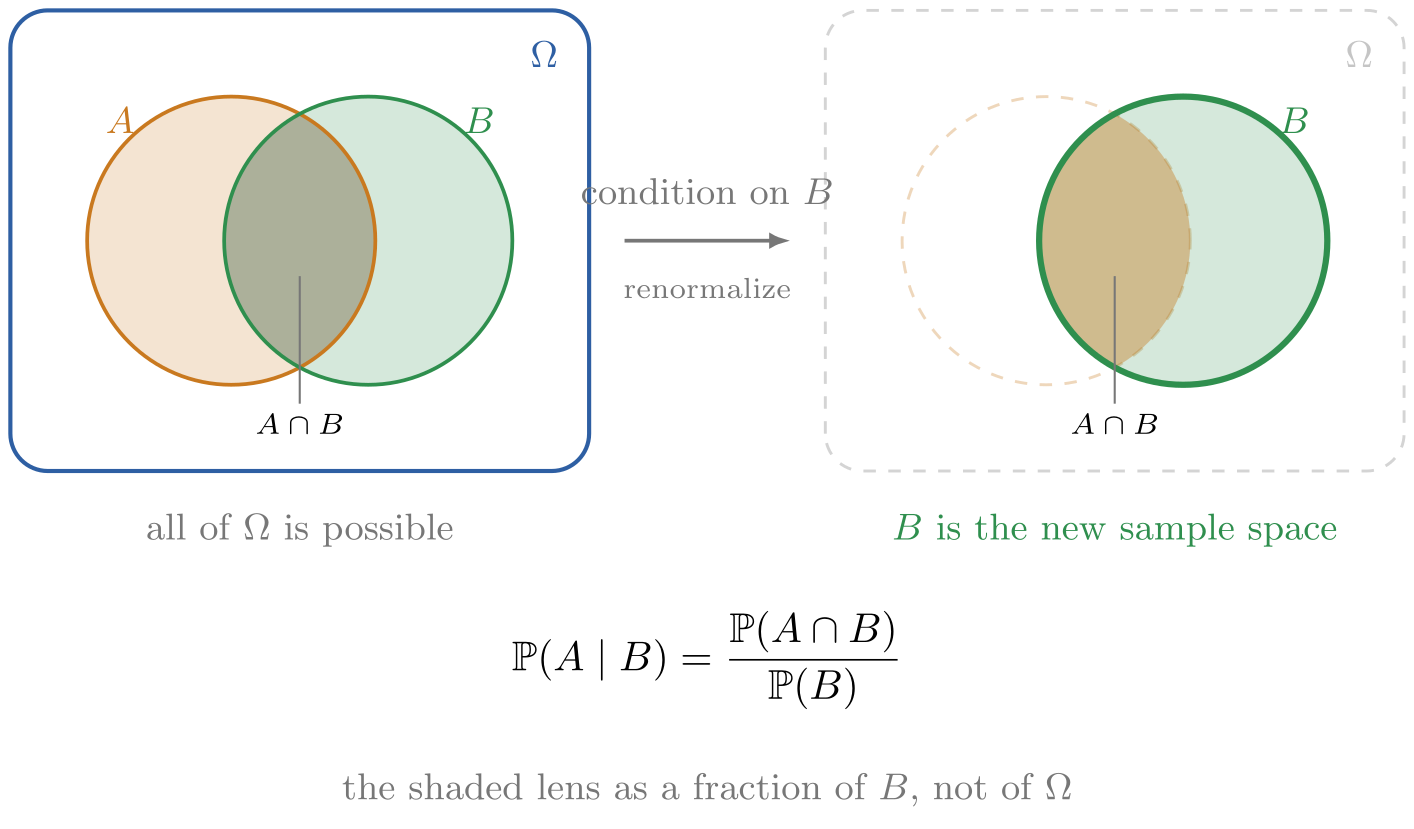
Then, definitionally speaking, the conditional distributionconditional distribution is defined as the ratio between the joint distributionjoint distribution of the two random variables (the one of interest, namely the next word, and the one that is being conditioned on, namely the previous words) and the distribution of the random variable that is being conditioned on, which corresponds with our intuition that the Venn diagram suggests:
- todo: bayes rulebayes rule
- todo: connect bayes rule over language to bayes rules over functions
and rearrange the identity for the joint, we have that
known as the product ruleproduct rule,
and reads that the probability of a t-length sentence is equivalent to the probability of the first t words multiplied by
the probability of t+1’th word occuring given the first t words occured.
The product rule is the probability of logical AND alongside the sum rule for the probability of logical OR.
The product rule is also referred to as the chain rulechain rule
given that we are chaining probabilities together,
and is the primary mechanism of generation within a large language model’s inference loop.
Morever, the fact that these distributions are functions
means that the division and multiplication in numpy are implemented via element-wise operatorselement-wise operation.
[!QUESTION]
np.ndarray’s to be? Prompt a language model to implement what you think. Pause, think and prompt!
Click to reveal answer
The type of is some function ,
or some np.ndarray with .shape (V, V, V, V, V).
If we had access to such distributions,
import numpy as np
history_VVVV = np.array_with_shape((V, V, V, V, V, V)) # t=4, i.e "Hello world, nice to"
joint_VVVVV = np.array_with_shape((V, V, V, V, V, V)) # t=5, i.e p("Hello world, nice to") AND p("you")
conditional = joint_VVVVV / history_VVVV # broadcast
1.4.3 Evaluation with Bias Variance Tradeoff
1.4 Parameterization Redux: Quantification
- why squared error loss from artem
Similarly to learning distributions from data, learning functions from data roughly follows the three step process of selecting a model for the task , a performance measure , and optimizing such measure on experience . Let’s take a look at the linearly modeling regression with squared error loss, a problem which straddles tools from all three languages of probability theory, linear algebra, and calculus.
For the task of house price prediction, the input space is the size in square feet, and the output space is the price, meaning that the function which needs to be recovered has the type of . An assumption about the structure of the data needs to be made, referred to as the inductive bias. The simplest assumption to make is to assume that there exists some linear relationship between the data and parameters so that ends up being modeled as an inner product plus bias, parameterized as :
One small adjustment we can make to is to fold the final bias term into the vector as , increasing the total dimensionality so that , and adjusting accordingly so that and . Then, the equation of our line with bias is simply parameterized as
Semantically speaking, each property of the input house is weighted by some weight , adjusted accordingly during the learning process so that it accurately reflects the property’s influence on the output price when evaluating a prediction . We can evaluate on all with a randomly intialized to ensure we’ve wired everything up correctly.
However, while specifying the equation of the linear regression model on paper screen
and subsequently evaluating the computation manually might have been sufficient
for pre-computational mathematicians such as Gauss and Legendre,
the discipline of statistical learning is entirely predicated on computational methods.
Let’s continue to use PyTorch’s core n-dimensional array datastructure with torch.Tensor,
this time modeling a function rather than some distribution :
(todo: maybe change example to closure following torch.nn)
{{#include ../../teeny/examples/2.2-regression.py:1:4}}
in which we can update the names of our torch.Tensor variables with the ranks of their vector
spacesReferred to as Shape Suffixes, described by Noam Shazeer, an engineer from Google
to clarify what dimensions these operations are evaluated on:
{{#include ../../teeny/examples/2.2-regression.py:5:8}}
and finally, actually enforce them via runtime typechecking with the jaxtyping package
(try swapping the return statements below to trigger a type error with the return type):
{{#include ../../teeny/examples/2.2-regression.py:9:19}}
Let’s now sanity-check that f_typechecked is wired up correctly
by evaluating it on all with random parameter w_D.
(todo: use actual housing data)
{{#include ../../teeny/examples/2.2-regression.py:29:41}}
random weight vector: tensor([-0.3343,  0.0768,  2.7828, -0.1331])
expected: $500000.0, actual: $-492.46
expected: $800000.0, actual: $-690.89
expected: $250000.0, actual: $-258.08
Clearly, these outputs are unintelligible, and will only become intelligible with a “good” choice of parameter .
Before we find such a parameter, let’s make one more modification to our function
to increase it’s performance.
Rather then evaluating f_typechecked on every input xi_D in the dataset zip(X_ND,Y_N) sequentially with a loop,
we can evaluate all outputs with a single matrix-vector multiplication by updating ’s function definition to the following
and the corresponding PyTorch updated to
{{#include ../../teeny/examples/2.2-regression.py:21:27}}
Now that we’ve selected our model for the task , we can proceed with selecting our performance measure which the learner will improve on with experience .
After the inductive bias on the family of functions has been made, the learning algorithm must find the function with a good fit. Since artificial learning algorithms don’t have visual cortex like biological humans[], the notion of “good fit” needs to defined in a systematic fashion. This is done by selecting the parameter which maximizes the likelihood of the data . Returning to the linear regression inductive bias we’ve selected to model the house price data, we assume there exists noise in both our model (epistemic uncertainty) and data (aleatoric uncertainty), so that where
prices are normally distributed conditioned on seeing the features with the mean being the equation of the line where , then we have that
TODO: generate prose/exposition by repaging lecture/text in ram
Returning to the linear regression model, we can solve this optimization with a direct method using normal equations. QR factorization, or SVD.
def fhatbatched(X_n: np.ndarray, m: float, b: float) -> np.ndarray: return X_n*m+b

if __name__ == "__main__":
  X, Y = np.array([1500, 2100, 800]), np.array([500000, 800000, 250000]) #  data

  X_b = np.column_stack((np.ones_like(X), X))              # [1, x]
  bhat, mhat = np.linalg.solve(X_b.T @ X_b, X_b.T @ Y)   # w = [b, m]

  yhats = fhatbatched(X, mhat, bhat) # yhat
  for y, yhat in zip(Y, yhats):
    print(f"expected: ${y:.0f}, actual: ${yhat:.2f}")
To summarize, we have selected and computed
- an inductive bias with the family of linear functions
- an inductive principle with the least squared loss
- the parameters which minimze the empirical risk, denoted as
Together, the inductive bias describes the relationship between the input and output spaces, the inductive principle is the loss function that measures prediction accuracy, and the minimization of the empirical risk finds the parameters for the best predictor.
1.5 Bias Variance Tradeoff
1.6 Summary
1.7 Further Reading
The primary texts consulted in the writing of this chapter were (Jurafsky and Martin 2026), (Eisenstein 2018), (Manning 2001), and (Cotterell 2024) for statistical natural language processing; (Bishop 2006) (Hastie, Tibshirani, and Friedman 2009), (Murphy 2022), (Mohri et al., 2018), and (Bach 2025), for machine learning more generally.
1.8 Problems
Intermezzo One: The Language of Probability Theory and Linear Algebra
As you now know from §1. Sequence Learning, language models are next token predictors.
Whether these language models are bigram models, logistic regression models, or the GPT-2 like neural nets that we will see in
Part II. Deep Neural Networks,
they are all functions that produce an output distribution over the next word given some input sentence as the history.
That is, they are functions of type
Before we dive into the internals of teenygrad itself in §2. The Tensor and implement our own framework capable of training the bigram and logistic regression models,
we will formally characterize our language model implementations from §1 using the language of calculus from high school, as well as probability and linear algebra which we will formally introduce now.
The one text which was heavily consulted over others was Formal Aspects to Language Modelling (Cotterell et al., 2024).
For more on formalization, please consult §A. From Problems to Proof.
I.1 Probability Spaces
Table of Contents (Intermezzo One)
Informally speaking, you intuitively understand the notion of a probability and a probability distribution. That is, a probability is a number between 0 and 1 that represents the chance, likelihood, or belief of some event happening, and a distribution is a list of such numbers. Probability distributions come from the concept of probability spaces, so before defining the former we must define the latter, which are measures of the size of sets.
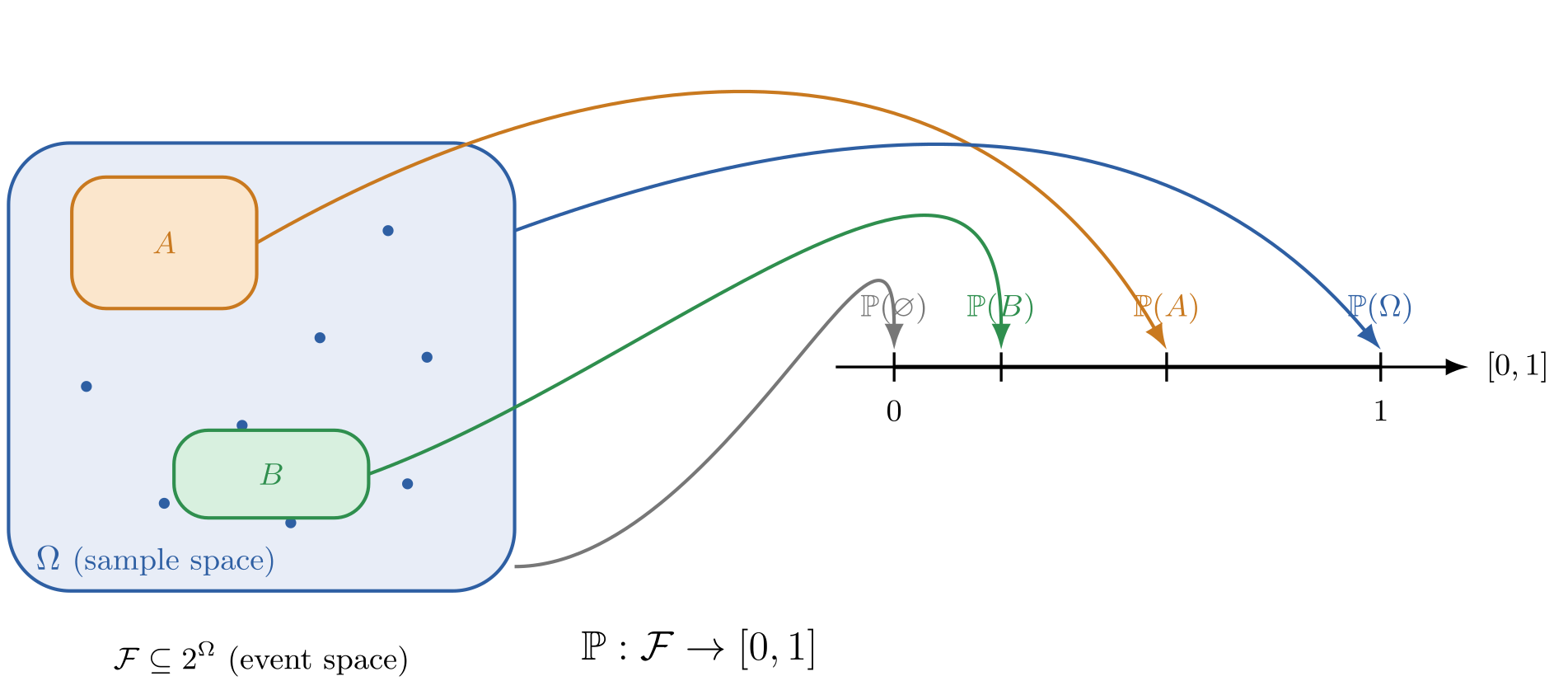 Figure I.1
Figure I.1 is comprised of three components. Namely, the blue box and it’s blue dots, the colored boxes, and the mapping from the colored boxes to the number line
- the sample space : the set of all possible outcomes in an experiment
- the event space : the set of all subsets in the sample space
- probability law : a mapping from the event space to a number between 0 and 1
Conceptually speaking, the language models we’ve seen in §1. Sequence Learning
such as GPT-2, the bigram model, and the logistic regression model which have type
produce (on a single evaluation) concrete probability distributions with np.ndarray
that come from
mathematically abstract probability spaces
where the sample space is the set of words in their vocabulary,
and their belief in a word occuring is represented by probability law defined on event space .
Caution
set()s for the sample space , the event space , nor define some functiondef probability_law(event_space: set) -> floatfor . They return a probability distributions, which we define in §I.2 Random Variables and their Distributions. Rather, the purpose of probability spaces as a mathematical definition is conceptual clarity with general definitionsDefining concepts without commiting to internal structure allows for a much broader class of objects to be considered. This is very much like type polymorphism (generics, traits, type classes), except the generality of mathematical concepts are usually “more” general than those that might be implemented with type polymorphism. For instance, this abstract definition of a probability space is generalized to cover any random experiment we’d like to model, from rolling dice, to generating language. However it’s quite unusual to have a program need to progam both. and rigorous results with theorems.
Let us now precisely define each component of a probability space , starting with the sample space .
A sample space is the set of all possible outcomes in an experiment denoted by ( code: \Omega).
- Consider flipping a coin. Then .
- Consider playing rock, paper, scissors. Then .
- Consider rolling a die. Then .
- Consider drawing a card. Then .
Consider generating a word from this very sentence. Then,
So conceptually speaking, language models like GPT2, the bigram model, and the logistic regression model
of type
which produce concrete distributions with np.ndarray on a single evaluation come from
mathematically abstract probability spaces where the sample space is the set of words in their vocabulary,
and their belief in a word occuring is represented by probability law defined on event space .
Important
An event space is the set of all possible subsets of the sample space denoted by ( code: \mathcal{F}).
TODO: something to say here about event spaces? cardinality of them?
A probability law is a function that sends an event to a number between 0 and 1.
Consider flipping a coin. Then we model the experiment with sample space , event space , and probability law
[!QUESTION]
A probability law is a function that sends an event to a number between 0 and 1, satisfying three axioms:
- non-negativity:
- normalization:
- additivity:
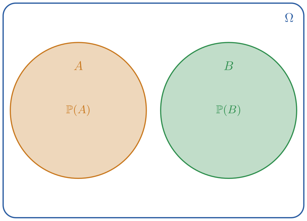
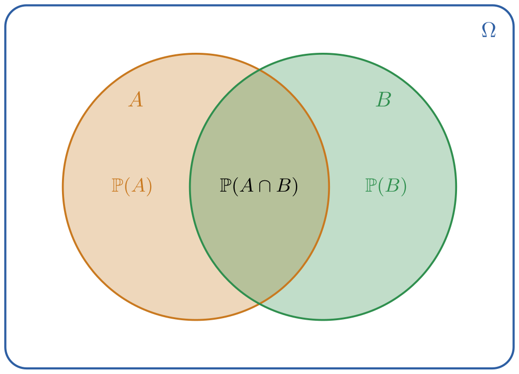
However the event which contains all foobarbaz is composed of overlapping events (corresponding to the right figure above), so the axiom of addivitiy does not apply. We can evaluate the union of non-disjoint (overlapping) events with the following corollary, known as the sum rulesum rule:
We have now sharpened our intuitive notion of chance, belief, and probability by formally defining them as the measure of the size of sets. These sets have a home, and the measure has a domain, namely the sample space and the event space and together with the probability law , comprise the definition of a probability space , albeit abstractly so. Let us now connnect this mathematically abstract space to the more concrete probability distributions we used in §1. Sequence Learning.
I.2 Random Variables and their Distributions
Table of Contents (Intermezzo One)
Probability distributions are the practical and concrete np.ndarrays we used throughout §1. Sequence Learning
when implementing the bigram and logistic regression language models.
So how do these connect to the abstract concept of probability spaces just defined?
The answer is with random variables and their probability mass functions,
which are functions that map outcomes to states, and from states to probabilities.
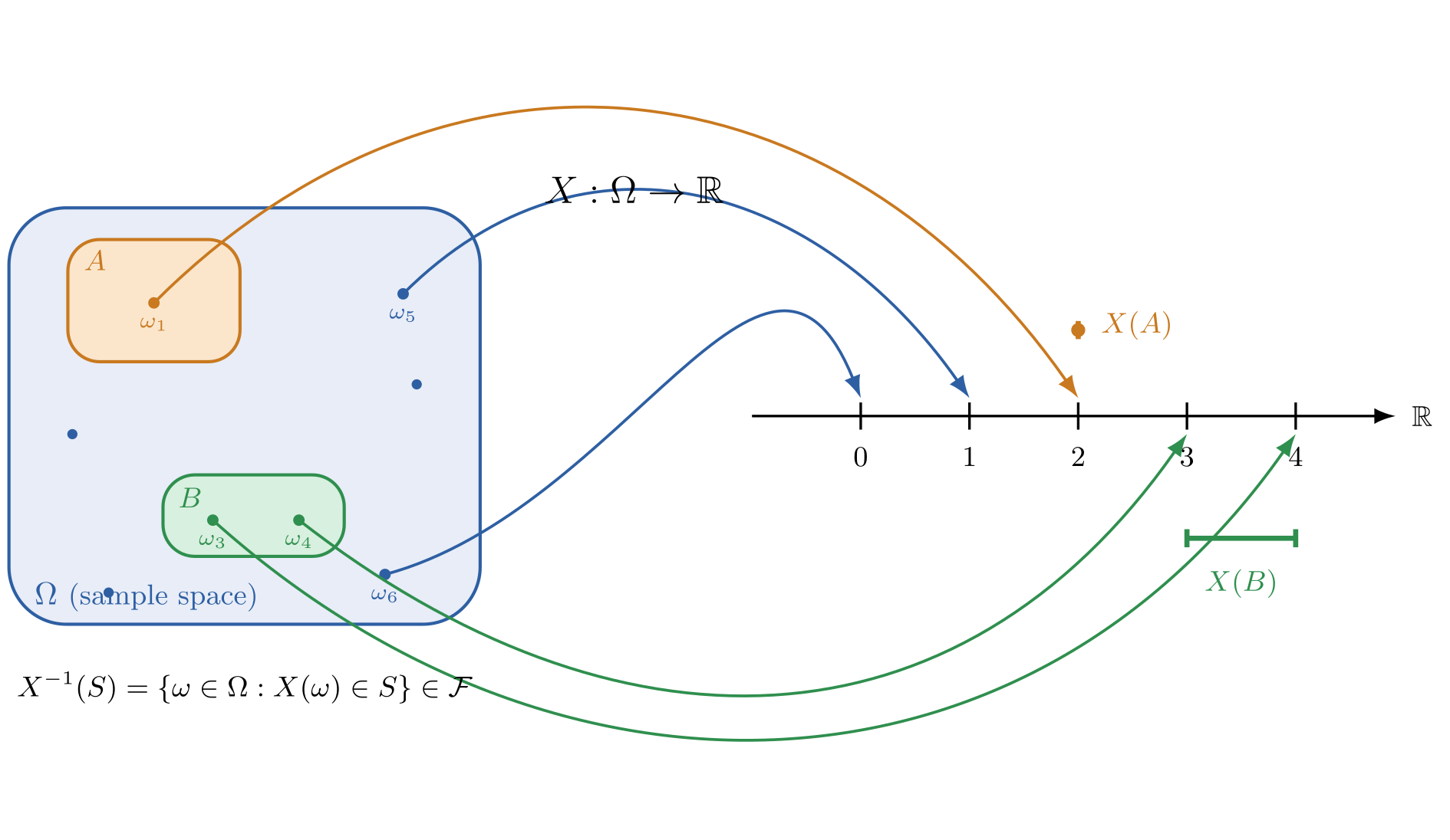
Figure I.2
(todo modify picture or include another picture to show distribution (probality assignment of variable taking on state))
Figure I.2 shows the same sample space and event space from §I.1 Probability Spaces, but rather than evaluate probabilities with the probability law by mapping events to the [0,1] number line (displayed in Figure I.1), we create one level of indirection with
- a random variable mapping outcomes in the sample space to states on the real number line and then defining
- a probability mass function mapping states to their probabilities.
So, starting with a sample space, you have to map outcomes to their state space with a random variable
before you can evaluate their probabilities with a probability mass function, rather than evaluate them directly with a probability law.
In other words, the two types are not equivalent .
For example, recall from §1.1 From Certain to Uncertain Knowledge
GPT-2’s np.ndarray output probs when passed the input string "Hello world, nice to":
import numpy as np

# GPT-2's output distribution when passed input "Hello world, nice to"
# Showing top 10 most likely words out of 50257.
tokens = [" see", " meet", " hear", " have", " be", " know", " you", " talk", " say", " get"]
probs = np.array([0.3169, 0.1268, 0.1246, 0.1046, 0.0471, 0.0352, 0.0320, 0.0128, 0.0114, 0.0067])
for i in np.argsort(-probs):
    print(f"{tokens[i]} : {probs[i]:.4f}")
Here, there is a random variable which maps outcomes from the abstract sample space to concrete states in state space . That is,
But notice the level of indirection with the random variable. All we’ve done is translate from sample space to state space. To obtain actual probabilities, we need to map from the state space to probabilities with the probability mass function . That is,
In other words, starting from sample space we compose with to obtain such that evaluating results in the probability of outcome . (todo. this is wrong?)
But how is the multidimensional array probs with support in related to the abstract concept of a probability space?
You may have noticed that the definition of looks quite similar to that of the probs:
import numpy as np
probs = np.array([0.3169, 0.1268, 0.1246, 0.1046, 0.0471, 0.0352, 0.0320, 0.0128, 0.0114, 0.0067])
This is because an alternative conceptualization of is some function
For conveniece sake we do store the outcomes in the tokens array so that we can print them next to their probabilities by looping over states with for i in np.argsort(-probs), but it’s important to note that is defined on real numbered states (represented with indices), and not on set-valued events. that has support in , or more accurately, With these two views, an alternative conceptualization of is some function
- todo: rvs map from one measurable space to another. we happen to like
On a single evaluation language models produce such probability mass functions
defined on a state space which are mapped over from an abstract sample space via random variable.
In practice, we forget about the concepts of sample spaces and random variables,
simply slugging around probability mass functions with np.ndarrays that have support in
n-dimensional Euclidean space, where n is the size of sample space.
In other words, we keep two as conceptual mathematical definitions without implementing them with code.
At this point, you may be wondering what is the point of the random variable’s indirection? … Now that you understand the notion of random variables and probability mass functions intuitively, let’s formally define them as concepts:
somehow motivate global view
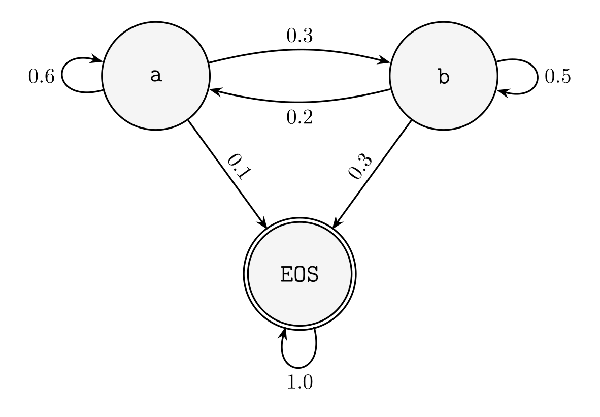
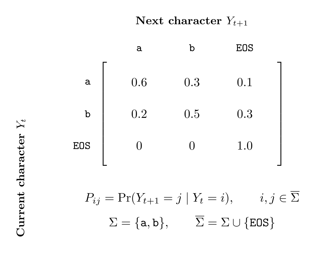
The intuition is very simple: every language model can be locally normalized. The precise formulation however, is not. proof with prefix probabilities
proof
however the converse direction is not a trivial result to establish examples
- 2 state model (markov chain), non-tight
- 2 state model (markov chain), tight (absorbs)
I.3 Probabilities of Sums, Products, Conditionals
I.4 Random Processes and their Kernels
Table of Contents (Intermezzo One)
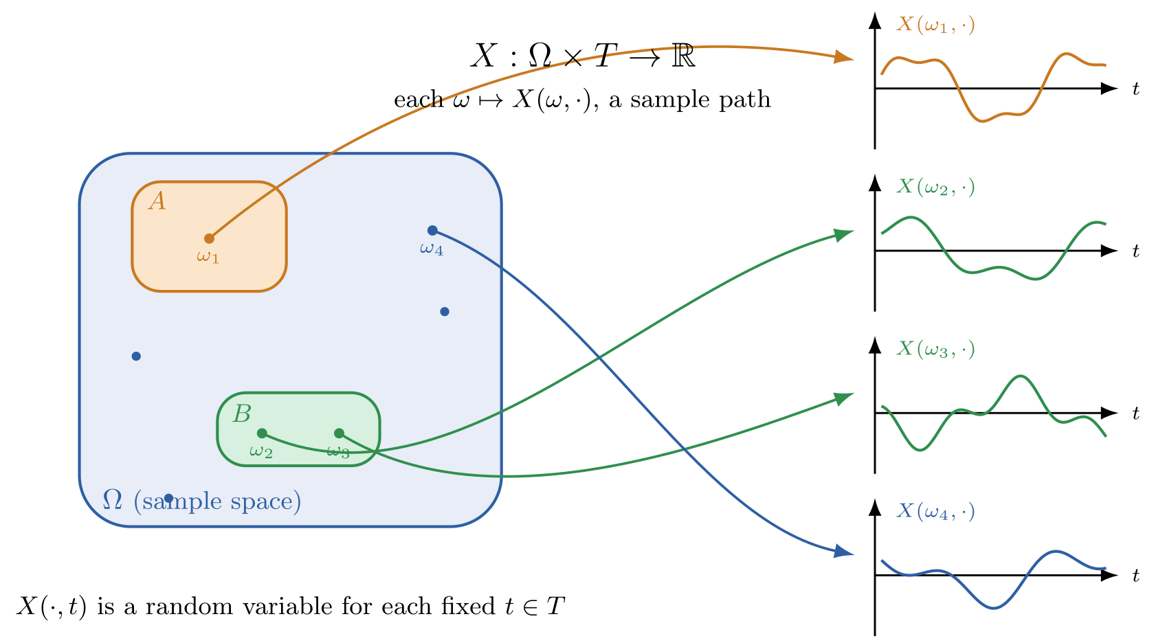
I.5 Measurable Spaces
I.6 Vector Spaces
Table of Contents (Intermezzo One)
I.7 Further Reading
The primary texts consulted in the writing of this chapter were (Bertsekas and Tsitsiklis 2008), (Chan 2021), (Wasserman 2004), and (Durrett (2019) for probability theory; (Strang 2026), (Strang 2019), and (Axler 2026) for linear algebra; (Boyd and Vandenberghe 2004) and (Kochenderfer and Wheeler 2019) for optimization.
2. From IPL’s Array to APL’s Multidimensional Array
2.1 From Virtual to Physical Machines (and Shapes)
- justify native for eager performance
- pyo3 https://github.com/j4orz/ateenysitp/blob/master/ARCHITECTURE.md#level-1-teenygrads-build-configuration-and-development-environment
- native components using cpython as encapsulation boundary
- freethreaded python eliminates multithreading problem
/// SGEMM with the classic BLAS signature (row-major, no transposes):
/// C = alpha * A * B + beta * C
fn sgemm(
  m: usize, n: usize, k: usize,
  alpha: f32, a: &[f32], lda: usize,
  b: &[f32], ldb: usize,
  beta: f32, c: &mut [f32], ldc: usize) {
  assert!(m > 0 && n > 0 && k > 0, "mat dims must be non-zero");
  assert!(lda >= k && a.len() >= m * lda);
  assert!(ldb >= n && b.len() >= k * ldb);
  assert!(ldc >= n && c.len() >= m * ldc);

  for i in 0..m {
    for j in 0..n {
      let mut acc = 0.0f32;
      for p in 0..k { acc += a[i * lda + p] * b[p * ldb + j]; }
      let idx = i * ldc + j;
      c[idx] = alpha * acc + beta * c[idx];
    }
  }
}

fn main() {
  use std::time::Instant;

  for &n in &[16usize, 32, 64, 128, 256] {
    let (m, k) = (n, n);
    let (a, b, mut c) = (vec![1.0f32; m * k], vec![1.0f32; k * n], vec![0.0f32; m * n]);

    let t0 = Instant::now();
    sgemm(m, n, k, 1.0, &a, k, &b, n, 0.0, &mut c, n);
    let secs = t0.elapsed().as_secs_f64().max(std::f64::MIN_POSITIVE);
    let gflop = 2.0 * (m as f64) * (n as f64) * (k as f64) / 1e9;
    let gflops = gflop / secs;

    println!("m=n=k={n:4} | {:7.3} ms | {:6.2} GFLOP/s", secs * 1e3, gflops);
  }
}
2.2 Accelerating the Communication of Hierarchies
Loop Reordering, Register and Cache Blocking
2.3 Accelerating the Computation of Pipelines
Instruction Level Parallelism via Loop Unrolling
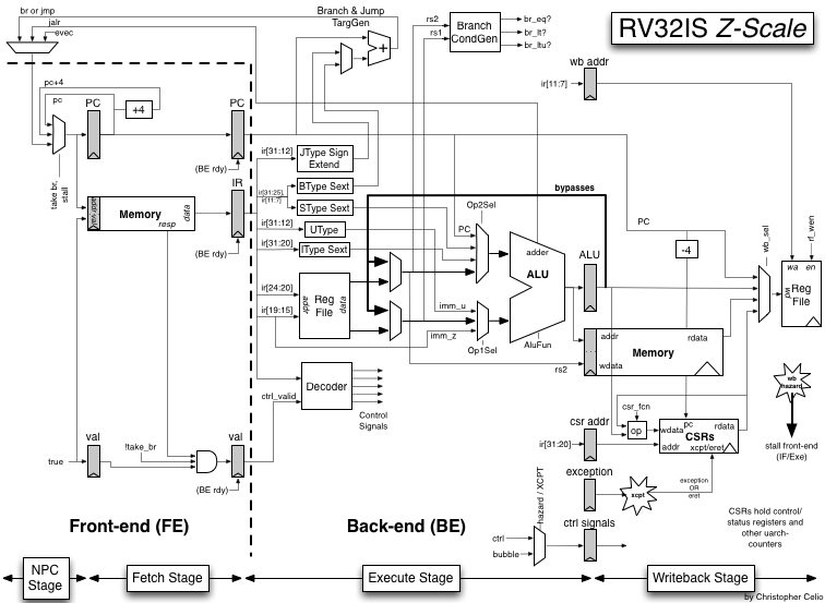
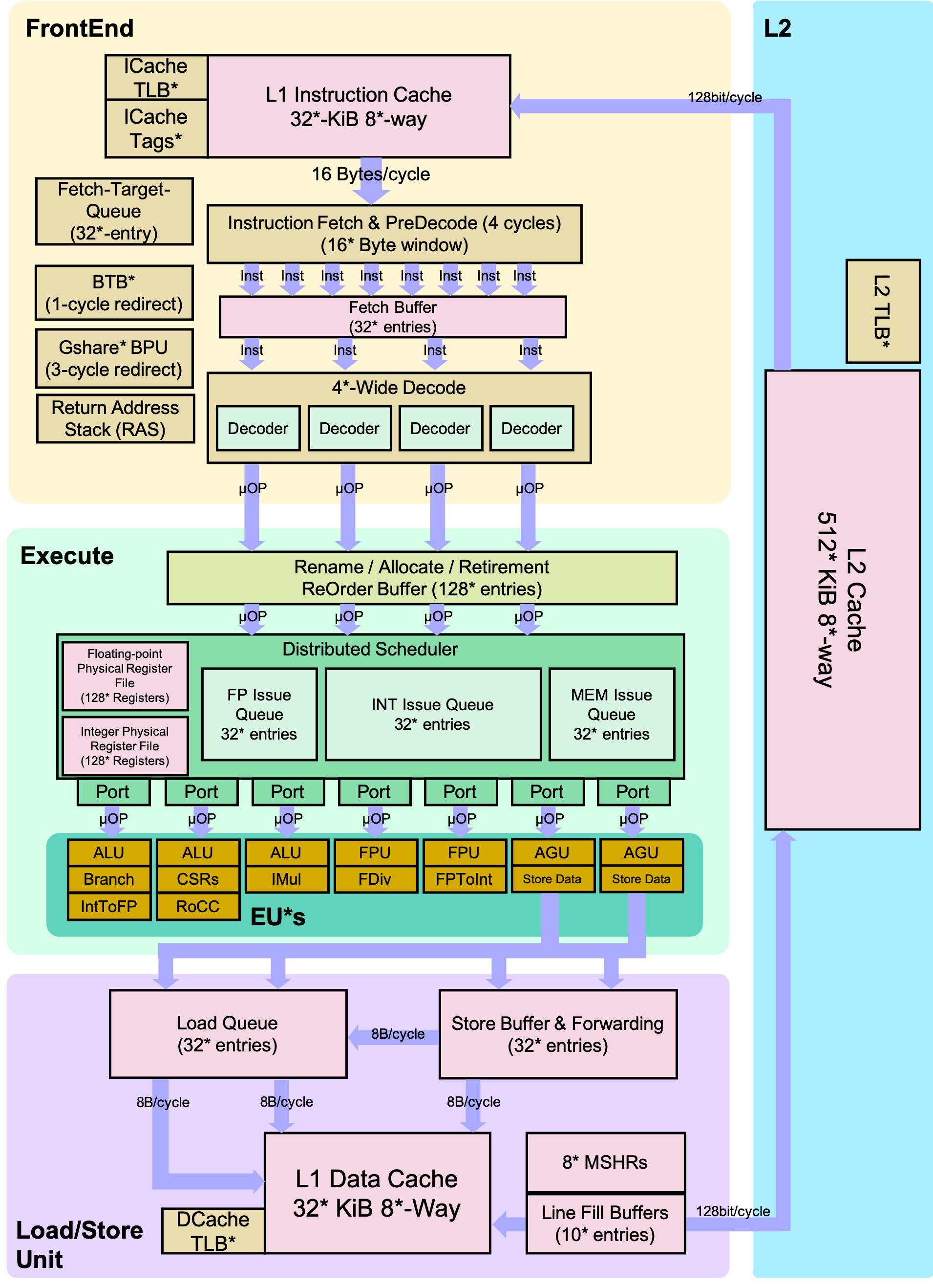
2.4 From Abstract to Numerical Linear Algebra
2.6 Summary
One quick way to summarize the milestones in high performance computing, compilers and architecture is to list the Turing Award winners: Alan Perlis (1966) for his influence on advanced programming techniques and compiler construction, including his role in designing ALGOL and establishing the discipline of programming languages as a field; John Backus (1977) for designing FORTRAN — the first high-level language to achieve widespread practical adoption — and formalizing language syntax through Backus-Naur Form; Tony Hoare (1980) for axiomatic semantics, giving programmers a formal logical framework for reasoning about program correctness; Niklaus Wirth (1984) for designing a sequence of clean, teachable languages — EULER, ALGOL-W, Pascal, and Modula — that shaped how programming languages are structured and implemented; John Cocke (1987) for pioneering optimizing compilers and the Reduced Instruction Set Computer (RISC) architecture, showing that simpler instruction sets allow faster hardware; William Kahan (1989) for fundamental contributions to numerical analysis, most consequentially the IEEE 754 floating-point standard that made reliable numerical computation reproducible across hardware; Frederick Brooks (1999) for landmark contributions to computer architecture — most notably the IBM System/360 — and for articulating the enduring lessons of large-scale software engineering; Frances Allen (2006) for foundational contributions to the theory and practice of optimizing compilers, including dataflow analysis and the program dependence graph; John Hennessy and David Patterson (2017) for a systematic, quantitative approach to designing and evaluating computer architectures, whose RISC principles underpin billions of processors and the open RISC-V standard; and Alfred Aho and Jeffrey Ullman (2020) for foundational contributions to programming language theory and compiler construction, most durably codified in the Dragon Book; and finally,Jack Dongarra (2021) for pioneering the numerical libraries — BLAS, LAPACK, and MPI — that became the substrate of high-performance scientific computing and modern deep learning accelerators;
2.7 Further Reading
The primary texts consulted in the writing of this chapter were